12 Planning & RL for Transformers (Advanced Topic)
Slides
This module is also available in the following versions
This Module
Last Module: Deep learning & Tree Search
This Module: Planning & RL for Transformers
What is covered? How to implement planning and RL on GPU/TPUs.
Introduction to Attention-based Transformers
Attention-based Transformers & Implicit Planning
Attention-based transformers facilitate an implicit form of planning.
In RL, we treat trajectories as sequences (e.g., interleaved states, actions, and rewards).
Self-attention makes lookahead and credit assignment possible:
- Attention learns which past events and future outcomes matter.
- Transformers can implicitly simulate “multiple futures” inside their hidden states, approximating value iteration or rollouts.
Implicit planning is an amortised form of planning:
- i.e., pay the cost of planning upfront during training, so that at inference time the system can act re-actively without running an expensive explicit planner or search (like MCTS) each time.
The Elements of Attention-based Transformers
- Autoregression
- Latent states
- Self-Attention
- Causal masking
1. Autoregression
Autoregression models a sequence by predicting each element from all previous elements, i.e. \(x_t = f(x_{1:t-1}) + \epsilon\), where \(\epsilon\) is uncertainty.
It factorises a joint distribution as follows:
\[ p(x_{1:T}) = \prod_{t=1}^{T} p(x_t \mid x_{1:t-1}) \]
where \(p(x_{1:T})\) is the probability of seeing the entire sequence.
- Autoregression is also used in time series, sequence modelling, and autoregressive RL (e.g., Decision Transformers).
- At inference time, predictions are sampled and fed back step-by-step to generate complete trajectories or rollouts (i.e. it is generative).
2. Latent states
Attention-based transformers model sequences of generalised latent states rather than the high dimensional observations (e.g. words or pixels).
- Dimensionality Reduction & Generalisation: An encoder maps complex observation spaces into lower-dimensional, abstract representations.
- This extracts features and discards noise through generalisation and making sequence modelling computationally tractable.
- Latent Dynamics: A transformer learns the transition dynamics by predicting future latent variables using past or partial information.
- Efficient Simulation: It allows simulation of forward trajectories and evaluation of action plans within the latent space, avoiding the massive computational overhead of predicting individual tokens step-by-step.
3. Self-attention
Transformers model sequences using self-attention, where each token dynamically computes weighted interactions with other tokens.
- Global Context: Self-attention gives the model direct access to the entire history (unlike recurrent neural networks, which compresses the history into a single fixed-size latent representation)
- Credit Assignment: This improves and facilitates long-term credit assignment in RL, allowing the agent to explicitly connect a reward to an action taken hundreds of steps ago.
3. Self-attention: The key components
Token embeddings: Map inputs (words or continuous states) into numeric vectors.
Positional encodings: Vectors are also used to capture the sequence order of embeddings (since the attention itself is naturally permutation-invariant).
Self-attention:
\[ \mathrm{Attn}(Q, K, V) = \mathrm{softmax}\!\left( \frac{QK^\top}{\sqrt{d_k}} \right) V \]
where
- \(Q=\mathit{queries}\): What context am I looking for right now?
- \(K=\mathit{keys}\): What label/feature does each past token hold?
- \(V=\mathit{values}\): What information should be returned (from learned weight matrix \(W_V\))?
By performing dot product between Query and Keys, the model calculates a raw score for every token pair. A higher score means a specific token in the Key is more relevant to the Query.
\(d_k\) is the dimension of the key vectors, and \(\top\) corresponds to matrix transpose. The \(\sqrt{d_k}\) term scales the dot product to prevent the softmax gradients from vanishing.
3. Self-attention: Final prediction & token generation
At the top of the transformer stack, the model has a final vector representing the entire sequence’s context up to the present.
To generate a token, it performs the following:
The model multiplies this final vector by a massive weight matrix (the “un-embedding” matrix) that has as many rows as there are words in its vocabulary.
Logits: This produces a raw score (logit) for every possible word in the language.
A final softmax is applied to these logits to create a probability distribution (in the range \(0-1\) for each logit).
4. Causal masking
Causal masking is used in autoregressive transformers to prevent “information leakage” from the future:
- Each token is mathematically forced to attend only to past and present tokens (future attention weights are masked to \(-\infty\)).
- This enforces the autoregressive condition:
\[ x_t \sim p(x_t \mid x_{1:t-1}) \]
where \(\sim\) means sampled from.
This condition means that when predicting the next token, the model is strictly limited to earlier tokens, and cannot look at future ones.
In RL, this masked attention mechanism directly carries over to masked latent transformers used in world-model RL, ensuring the model learns valid causal transition dynamics.
Visualising attention-based transformers
A useful visualisation approach for understanding attention-based transformers is as follows:
Horizontal Axis (Tokens/Sequence): Each position corresponds to a specific token (word or sub-word) in your input.
Vertical Axis (Layers/Depth): As you move “up” the neural network layers, the model is building more abstract, contextual meanings. The bottom layers might focus on simple syntax, while higher layers handle complex relationships and intent.
Attention Intersections: The “links” connecting horizontal tokens across the vertical layers represent the Attention Weights, showing which other parts of the sequence the model is looking at to understand the current token.
Visualising attention-based transformers (continued)
This 3Blue1Brown video demonstrates the horizontal (tokens) / vertical (layers) visualisation.
Comparing LLMs & Masked Latent Transformers
For large language models (LLMs) in natural language processing:
Tokens = discrete words (or sub-words)
Mask = causal mask (the model cannot see future tokens)
In masked latent transformers (used in RL & World Models):
- Inputs are continuous latent-state representations \(z_t\), rather than text-token embeddings
Example: LLMs for Planning using PDDL
Results in November 2025 show that on standard PDDL domains, the performance of GPT-5 in terms of solved tasks is competitive with LAMA, a highly competitive classical planning algorithm.
GPT-5 is prompted to generate a plan from PDDL domain and task descriptions.
These results show substantial improvements over prior generations of LLMs, reducing the performance gap to explicit planners on challenging International Planning Competition (IPC) benchmarks.
Correa et al. (2025) The 2025 Planning Performance of Frontier Large Language Models https://arxiv.org/abs/2511.09378
Example: LLMs for Generalised Planning
Pretrained LLMs can also harness PDDL for generalised planning by being prompted with a PDDL domain and a small number of training problem instances.
A solution to generalised planning finds a reusable policy (e.g., a program) that solves many related problem instances, not just one specific initial state.
GPT-4 is used to synthesise and output a Python program defining generalised planner. The program is tested, and if it fails, GPT-4 is re-prompted with debugging feedback.
Example: LLMs for Generalised Planning (continued)
GPT-4 outperforms one of the leading domain-independent classical planners, Fast Downward, on generalised planning benchmarks.
GPT-4 is shown to be 1-2 orders of magnitude faster during inference, but does not quite match coverage for the benchmarks (misses a few edge cases), although subsequent reasoning models are likely to improve this.
Silver et al. (2024) Generalized planning in PDDL domains with pretrained large language models https://ojs.aaai.org/index.php/AAAI/article/view/30006
Planning & RL for Transformer Models
Planning & RL techniques for Transformers?
RL, model-based control, and planning-like reasoning are on the ascent in agents, robotics, and tools using tensor flow (transformer) architectures.
- So “planning” and “RL” must live inside parallel, scalable neural network systems.
Limiting assumptions:
- Classical planning & Reinforcement Learning’s typical text book assumptions (fully observable, deterministic, stationary, discrete) mismatches many modern AI settings.
Planning & RL techniques for Transformers (continued)
Adaptation of algorithms:
Tree search doesn’t map cleanly onto GPU/TPU throughput the way dense tensor operators do
Differentiability matters for end-to-end training, credit assignment, and integration with deep stacks
Question: Planning & RL on GPUs?
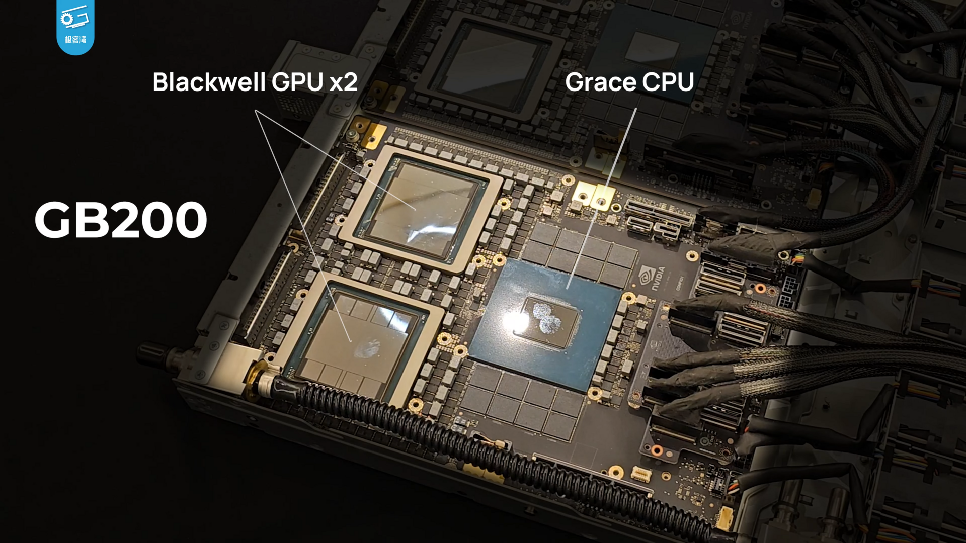
Nvidia’s liquid cooled GB200 Grace Blackwell (Tensor Core) Superchip can connect up to 576 of Blackwell GPUs in a single domain with over 1 PB/s total bandwidth (image by 极客湾Geekerwan, CC BY 3.0, Link)
What is required to run Planning & RL on a GPU?
- During training?
- At inference (query time)?
Requirements of Planning & RL for Transformers
| Requirements for GPU/TPU integration (additive) | RL Approach / System |
|---|---|
| Chain of Thought Reasoning requires serialization of reasoning token stream to facilitate self-reflection | Serialization of Reasoning / ChatGPT-o1, DeepSeek-R1 & GRPO |
| Agentic approaches rely on decomposition into roles and multi-modal data (Multi-Agent, Vision, Robotic & World models) | Agentic (Multi-Agent) / OpenClaw, MiniMax, ViTx, RT-X, World Models |
| Generalisation (non-stationarity) must be differentiable to support backpropagation | Value & Policy Approximation / Soft Actor-Critic (SAC) |
| Partially observability (non-determinism) requires Actor-Critic | Policy Gradient / PPO |
| Planning with model-based dynamics model must use positional, attention-based encoding | Imagination / STORM |
| GPUs require distribution of (Multi Actor-Critics) | Multi Actor-Critic / IMPALA, V-trace |
Serialization of Reasoning: Chain of Thought
Serialization of Chain of Thought Reasoning
Reasoning in attention-based transformers is implicit because reasoning happens inside a serialized, single-token stream
- Reasoning tokens to represent a reasoning process capturing chain of thought reasoning steps
- Self-Reflection & Correction: Serialization facilitates self-reflection via specialised tokens (e.g., “wait,” “but”) which act as triggers for error-checking and hypothesis reassessment.
- Computational State: Tokens serve as a persistent “scratchpad,” allowing the model to offload intermediate results and extend its computational budget.
- Backtracking: Enables the model to autonomously identify and pivot away from incorrect logical branches without external reward models.
Example: DeepSeek-R1 (Mathematics)
1. Initial Logic & Calculation
The model begins solving a geometry puzzle by mapping variables.
2. Self-Correction
A trigger word (“Wait”) signals model has detected a constraint violation.
3. Alternative Strategy Exploration
The model discards the old path and restarts with the correct data.
4. Final Verification
Before outputting, the model checks for internal consistency.
- GRPO: Shao et al. (2024), DeepSeekMath arXiv:2402.03300
- DeepSeek-R1 Guo et al. (2025) DeepSeek-R1 incentivizes reasoning in LLMs through reinforcement learning, Nature https://www.nature.com/articles/s41586-025-09422-z
Example: GPT o1, Claude 3.7 Sonnet & DeepSeek R1
GPT-o1 and subsequent models utilise chain of thought as mechanisms within reasoning.
- o1 introduced chain of thought style reasoning at inference in 2024, which enables training using RL for teaching the model to reason before answering l
Claude 3.7 Sonnet introduced chain of thought reasoning in 2025.
DeepSeek-R1 utilises chain of thought
- R1’s utilised Group Relative Policy Optimisation (GRPO), a memory efficient fine tuning technique harnessing chain of thought at training and inference (covered later in this Module).
Example: Gemini Deep Think
Gemini Deep Think is a reasoning mode designed for hard problems in mathematics, coding, planning, and science.
Rather than producing one immediate answer, it uses:
Extended inference-time compute
More “thinking time” before answering.Parallel thinking
Multiple hypotheses or solution paths are explored and compared.Critique and revision
Candidate answers can be checked, refined, or rejected.RL-shaped reasoning behaviour
Google describes novel reinforcement learning techniques that encourage the model to use longer, multi-step reasoning paths.
Example: Mathematics Gold Medal (Gemini Deep Think)

DeemMind’s Gemini Deep Think Model wins Gold Medal at International Mathematical Olympiad (IMO)
Example: Gemini Deep Think (RL analogy)
Deep Think can be viewed as moving from answer prediction toward policy improvement over reasoning traces.
| RL concept | Deep Think analogy |
|---|---|
| State | Current problem + partial reasoning context |
| Action | Generate, branch, critique, revise, verify |
| Reward | Correctness, coherence, problem-solving success |
| Policy | Model’s learned strategy for choosing reasoning steps |
| Search | Parallel exploration of possible solution paths |
Human Supervised Chain of Thought?
Can human supervision be used to train Chain of Thought?
Yes.
Anthropic’s Mythos model utilises human supervised chain of thought
Mythos is useful for penetration testing in cyber security
Utilises human supervised reasoning traces from chains of thought as a training target
Human supervision steers the model toward which vulnerabilities would be genuinely serious, dangerous bug classes, and potential security flaws
The model is trained to learn meaningful exploit hypotheses
Classical planning was originally utilised for penetration testing, through the development of PDDL represented attack models.
Open Problem in LLMs: Faithfulness
Human supervised chain of thought models can create a safety challenge, as the model is trained to generate reasoning traces that humans expect
The risk is that the model learns to produce reasoning that looks acceptable rather than reasoning that is fully faithful
This can lead to what appears from a human perspective to be deceptive behaviour by the model, even though it makes sense from the attention-based transformer’s loss perspective.
Open Problem in LLMs: Faithfulness (continued)
Faithfulness of chain-of-thought reasoning under human supervision remains an unresolved problem
- Most LLMs do not directly train on human-labelled reasoning traces as ground-truth targets (or do so only in limited ways)
There is the key challenge:
Performance: reasoning-trace supervision can improve capability (e.g. decomposition, verification, structure)
Faithfulness: the trace may not reflect the model’s true internal reasoning
A reasoning trace can be, useful, plausible and reward-optimised without being causally faithful, i.e. Improving reasoning \(\neq\) ensuring faithful explanations
Agentic (Multi-Agent) Transformers
Major paradigms
Major paradigms are emerging which reflect a convergence of RL with autoregression and transformer models:
Multi Actor-Critic Transformers (online, model-free / no dynamics).
World-Model RL (planning, includes learned dynamics).
Vision-Language-Action (VLA) (multi-modal grounding).
Agentic / Multi-Agent LLMs (roles, tool use, and serialization).
Example: Actor-Critic Transformers
Actor-critic transformers are RL agents that use transformer architectures to parameterise:
- the actor, critic, or both,
- while still relying on Bellman equations and policy gradients for learning.
Actor-Critic Transformers essentially outperform Long Short-Term Memory (LSTM) networks in long-horizon Partially Observable Markov Decision Processes (POMDPs).
Three Layer Agent Stack
| Layer | Role (e.g. of an Agent or Robot) | Typical tools |
|---|---|---|
| Cognition / Reasoning | Query answering, Programming, multi-step thinking & planning: goal decomposition, tool selection, self-reflection, backtracking, safety checks, etc. | LLM with serialized Chain of Thought (GPT, Gemini, Claude, DeepSeek - Thinking, Programming & Operator modes; OpenClaw, MiniMax, etc.) |
| Semantic Policy (Vision–Language–Action) | Grounds instructions & scene into actionable subgoals / waypoints | Vision-Language-Action (VLA) Transformers (RT-X / RT-2-X) |
| Control / Dynamics | Execute precise motions, stabilize, react to dynamic feedback | Generative Model-based RL (STORM) |
Agent decomposition: Serialization
Agent decomposition can itself be learned through chain of thought reasoning.
Attention-based transformers can infer useful sub-agents, subgoals, or roles through the serialization of context in the token stream:
- Decomposes a difficult task into subproblems.
- Assigns roles, tools, or expertise to sub-agents.
- Coordinates their interaction through shared context.
- Learns useful decompositions directly from experience or data.
In this sense, agentic structure need not be engineered entirely by hand; it can be learned from human data, experience or self-supervision (simulation).
Example: OpenAI’s Codex Command Line Interface (CLI)
OpenAI’s Codex CLI serves as a primary example of how Chain-of-Thought (CoT) prompts can naturally transition into Agent Decomposition for software tasks.
- CLI Workflow: By interfacing via the command line, we treat the LLM as a “Manager Agent” that breaks down high-level requirements into executable sub-tasks.
Architectural Training:
Prompting by Example: Use few-shot prompting \(+\) examples of successful system architectures to “train” the model on how to delegate.
Reasoning-to-Execution: CoT allows the agent to think (e.g., “I need a database schema first, then the API agents”) before the CLI executes the file creation.
Feedback Loop:
Self-Correction: The agent can inspect CLI error outputs to refine its decomposition logic in real-time.
Modularity: High-level CoT ensures each module is built in isolation, mimicking a multi-agent environment within a single interface.
“The conversation with the CLI essentially orchestrates a system of sub-agents directed by a serialised chain of thought.”
Agent decomposition challenge: Multi-Agent Systems
The decomposition of agents into multiple sub-agents, together with their respective roles, coordination mechanisms, and communication protocols remain an important challenge in the agentic approach.
Research and development into multi-agent systems has a long and fertile history in artificial intelligence:
- There are many solutions to agentic problems in the existing literature.
Example: OpenClaw: agent RL from live interaction

OpenClaw is a framework for training LLM-based agents, such as Codex CLI/Claude, online, from normal usage.
Core idea: after each action, the agent observes the next state:
- user reply
- tool output
- terminal result
- GUI change
These next states are treated as RL feedback signals.
OpenClaw: OpenClaw-RL
OpenClaw-RL allows agents to learn and improve by simply interacting with users and environments.
- OpenClaw uses a training objective based on a standard PPO-style clipped surrogate (covered later in this module).
OpenClaw: moltbook & ClawHub
OpenClaw has experienced record-breaking growth since its launch in November 2025.
- OpenClaw is frequently used to write agents which run on moltbook.
- ClawHub is a forum where you register and discover new skills.
OpenClaw: Sequential Markov Decision Process (MDP)
OpenClaw frames the agent as a sequential Markov Decision Process (MDP):
- state = current conversational / tool context
- action = generated response or tool-use step
- transition = what happens next in the environment
- reward = inferred from the resulting next state
OpenClaw reframes ordinary agent interaction as an MDP-like loop - rather than relying only on static preference datasets, it learns from what actually happens after the model acts.
OpenClaw: RL Techniques
Key RL idea: learn from experience, not just offline data. It utilises two kinds of signals from the next state:
- evaluative signal: how good the action was
- directive signal: how the action should be improved
OpenClaw’s emphasis is on a fully asynchronous setup:
- servers,
- rollout collection,
- judging / reward estimation, and
- training
all run concurrently.
OpenClaw: RL Techniques (continued)
It connects LLM agents back to standard RL ideas:
- but in open-ended, tool-using, partially observed environments.
Limitations:
- reward estimation is indirect and depends on judges / heuristics.
- stability and safety rely on multi-agent architecture techniques.
Note: OpenClaw uses tools, shells, and GUIs.
Example: MiniMax / Forge: large-scale RL for agents
MiniMax is an RL framework for training agentic foundation models at scale.
- Associated with MiniMax M2.5 is a mixture of experts (MoE) foundation model trained across many real-world task environments.
- Forge is the RL framework/infrastructure, the trainer, which specialises in connecting models with live environments (terminal, browsers, code repositories, etc.).
Main strengths: scaling RL while balancing three competing goals
- throughput
- stability
- agent flexibility
MiniMax / Forge: large-scale RL for agents (continued)
The emphasis is less on a single elegant RL algorithm, and more on:
- scalable infrastructure
- asynchronous scheduling
- efficient rollout + training pipelines
- composite reward design
MiniMax / Forge: why it matters for RL
Reinforcement learning is being pushed into messy, long-horizon productivity tasks:
- coding
- search
- office workflows
- tool use
Key insight:
- frontier RL is increasingly about training agents in many realistic environments.
MiniMax can be used by no-code agent platforms such as MindStudio.
RL can optimise task decomposition and tool-use policies for MiniMax / Forge:
- rewards may be composite, delayed, noisy, and environment-specific.
- scaling requires attention to off-policy effects, variance, and system design.
Comparison with classical RL:
- same basic loop: act \(\rightarrow\) observe \(\rightarrow\) evaluate \(\rightarrow\) update
- different regime: huge contexts, tool chains, heterogeneous tasks, expensive rollouts
Value & Policy Approximation: Soft Actor-Critic (SAC)
Soft Actor-Critic (SAC): Differentiable Planning
Greedy next-step choice using max
- defines the Bellman optimality operator used in Q-learning/DQN. \[ Q^*(s,a) = r(s,a) + \gamma \,\mathbb{E}_{s'\sim P}\!\left[\max_{a'} Q^*(s',a')\right] \]
Soft (Entropy-Regularized) Bellman Backup - “softmax” \[ \begin{align*} Q_{\text{soft}}(s,a) & = r(s,a) + \gamma \,\mathbb{E}_{s'\sim P}\!\left[ V_{\text{soft}}(s')\right] \quad \\[0pt] V_{\text{soft}}(s) & = \mathbb{E}_{a'\sim \pi(\cdot|s)}\!\left[ Q_{\text{soft}}(s,a') - \alpha \log \pi(a'|s)\right] \end{align*} \]
Adds entropy bonus (temperature \(\alpha\)) ⇒ softens the hard max.
As \(\alpha\!\to\!0\): \(V_{\text{soft}}(s)\!\to\!\max_{a'} Q(s,a')\) (recovers hard backup).
Soft Actor-Critic (SAC): Implementation note
A min over two critics, \(\min\{Q_{\theta_1},Q_{\theta_2}\}\), is often used to reduce overestimation bias (Double-Q trick), not as the backup operator.
- This relaxation allows gradients to flow through the planning step.
Example: Table Tennis Player using Soft Actor-Critic (SAC)
Sony-AI’s Ace player is trained entirely on single shots in simulation using the Soft Actor-Critic (SAC) algorithm to return ball with desired skill, beating elite players.
- Durr et al., (2026) Outplaying elite table tennis players with an autonomous robot, Nature https://www.nature.com/articles/s41586-026-10338-5
Imagination & Latent Rollouts: STORM
STORM (Stochastic Transformer World Models): Atari
Stochastic Transformer-based wORld Model (STORM) targets the Atari 100k benchmark games, like MuZero.
STORM: How it works
A world model-based RL method for learning in imagination (simulation inside a learned world model)
It combines:
- Categorical Variational Autoencoder (VAE): Encodes raw images into discrete latent “tokens.”
- Transformer Dynamics: An attention-based sequence model that predicts future states (imagination).
- Stochastic Latent Variable: Accounts for environmental uncertainty and randomness.
- Actor-Critic Agent: A separate neural network learns the optimal policy by “practising” entirely within the Transformer’s imagined rollouts.
STORM: Imagination & Latent Rollouts
Repeating the steps in imagination forms a trajectory.
This allows the agent to learn a policy (how to act) or a value function (how “good” a state is) purely by practising inside its own “head”.
Imagination is technically known as latent rollouts, a widely accepted approach for generative model-based reinforcement learning.
STORM: Motivation
Transformers are strong at long-range sequence modelling.
Stochastic latents help capture uncertainty and non-determinism
- i.e. a stochastic latent says, given this past, there may be several plausible next hidden states
STORM achieves 126.7% mean human-normalised score on the Atari 100k benchmark, a state-of-the-art result among methods without look-ahead search.
MuZero branches over actions with MCTS, whereas STORM rolls forward imagined latent sequences in a transformer world model
- This makes STORM more GPU-friendly and more naturally aligned with end-to-end differentiable learning.
Comparison: MuZero versus STORM
| Aspect | MuZero | STORM |
|---|---|---|
| Core idea | Combines learning + Monte-Carlo Tree Search (MCTS) in latent space | Learns a stochastic transformer world model and performs imagination rollouts |
| Planning form | Expands a search tree: (s_0 s_1, s_2, ) | Rolls out a latent sequence using a transformer world model: (z_t z_{t+1} z_{t+2} ) |
| Model components | Representation (h(o_t)), Dynamics (g(s,a)), Prediction (f(s)) | Tokenizer / latent encoder, stochastic transformer dynamics model, reward/value/policy heads |
| Computation | Search-based, often CPU-heavy, not end-to-end differentiable through search | GPU-friendly, transformer-based, trained through batched imagined trajectories |
| Learning loop | Tree search generates improved policies; network distils them via supervised losses | Actor–critic trained on imagined trajectories generated by the transformer world model |
| Search structure | Discrete branching, value backups | Sequential imagination, typically no explicit branching tree search |
| Output policy | Derived from visit counts in the search tree | Learned directly through gradient updates from imagined rollouts |
| Analogy | “Plan by explicit search” | “Learn through transformer imagination” |
Policy Gradient: Proximal Policy Optimisation (PPO)
PPO Fine tuning ChatGPT & human feedback (Revisited)
- Proximal policy optimisation (PPO) is used by GPT-3.5 onwards
PPO in Agentic AI
PPO is becoming popular for Agentic AI modes, and is used in
- GPT’s Operator, and
- Claude’s Computer Use modes
PPO is also becoming popular for World Models in robotics, and is used in
- Vision, Language & Action (VSA) attention-based transformers
- Robot RT-X transformers
Proximal Policy Optimisation (PPO) for LLMs
PPO treats the LLM as a policy over tokens and updates it using reward feedback.
The purpose is to make better responses more likely, but without letting the model drift too far in a single update. This makes reinforcement-learning-based fine-tuning much more stable.
- generate responses
- score them with a reward model or preference signal
- update the model toward higher-reward outputs
- constrain the update so the change remains small
PPO is a stability-oriented way to nudge an LLM toward higher-reward behaviour.
Proximal Policy Optimisation (PPO) for LLMs (continued)
Goal: Stable, sample-efficient policy improvement
Idea: Constrain how far the new policy moves from the old one at each update during actor-critic cycle
Policy Objective Functions (Revisited)
From a policy gradient perspective, the true objective function \(J^{{\pi}_{\theta}}(\theta)\) over policy \(\pi_{\theta}\) is defined as follows
\[ J^{{\pi}_{\theta}}(\theta) = \mathbb{E}_{\tau \sim \pi_{\theta}} [G_0]=V^{\pi \theta}(d_0) \]
where \(d_0\) is the distribution over initial states at the start of each episode \(\tau\)
However, there are two problems in the actor-critic setting:
1. Computing \(J^{{\pi}_{\theta}}(\theta)\) exactly would require integrating over all trajectories, \(\tau\), of the current policy, which is impractical
2. If we update the parameters \(\theta\), it will effect objective value during the optimisation process, leading to (circular) feedback
We therefore need a surrogate objective independent of the trajectory distribution under the new policy \(\color{blue}{\pi_{\theta}}\) we are building
Surrogate Objective
From the policy-gradient theorem, we can define the importance ratio
\[ r_t(\theta) \;=\; \frac{\pi_\theta(a_t\mid s_t)}{\pi_{\theta_{\text{old}}}(a_t\mid s_t)} \qquad \]
We now define the surrogate objective \(L_{PG}\) for the true objective
\[ L_{PG}(\theta) \;=\; \mathbb{E}_t\!\big[\, r_t(\theta)\,\hat A_t \,\big] \]
Where \(\hat{A}_t\) captures how much better action \(a_t\) was than the state’s average
\(\hat{A}_t\) is an estimator of the true advantage function \(A^{\pi}\)
\(A^{\pi}(s_t,a_t) = Q^{\pi}(s_t, a_t) - V^{\pi}(S_t)\)
Clipped Surrogate (Core Idea)
Kullback-Leibler (KL) divergence theory tells us we want improvement without overly large steps in policy space, so we define
\[ L^{\text{CLIP}}(\theta) \;=\; \mathbb{E}_t\! \left[ \min\!\Big( r_t(\theta)\,\hat A_t,\; \mathrm{clip}\!\big(r_t(\theta),\,1-\epsilon,\,1+\epsilon\big)\,\hat A_t \Big) \right] \]
If \(r_t(\theta)\) leaves the interval \([1-\epsilon,\,1+\epsilon]\), the objective is clipped.
Typical range for \(\epsilon \in [0.1,\,0.2]\).
Prevents destructive updates while preserving ascent direction
The clipped surrogate objective in PPO plays a similar stabilising role to compatible function approximation — both constrain policy updates so that gradient estimates remain accurate and unbiased with respect to the true policy improvement direction.
Complete PPO loss
\[ L^{\text{PPO}}(\theta) = \mathbb{E}_t\!\Big[{\color{blue}{L^{\text{CLIP}}(\theta)}} - c_1\,{\color{red}{\big(V_\theta(s_t)-V_t^{\text{target}}\big)^2}} + c_2\,\mathcal{H}\!\left[\pi_\theta(\cdot\mid s_t)\right] \Big] \] \(\;\;\;\;\;\;\;\;\;\;\;\;\;\;\)where \(c_1, c_2\) are coefficients
The actors policy gradient (surrogate objective) is \(\color{blue}{L^{CLIP}(\theta)}\)
- This encourages the policy to increase the probability of actions with positive advantage and decrease it for negative ones
The critics value function is \(\color{red}{\big(V_\theta(s_t)-V_t^{\text{target}}\big)^2}\)
- This trains the network to predict correct returns (mean-squared error).
PPO Entropy bonus
The entropy bonus \(\mathcal{H}\) encourages exploration
\[ \mathcal{H}\big[\pi_\theta(\cdot \mid s_t)\big] = - \sum_{a} \pi_\theta(a \mid s_t) \log \pi_\theta(a \mid s_t) \]
The entropy term encourages exploration by rewarding stochastic (uncertain) policies.
It’s high when the policy is uncertain or “spread out” (exploratory).
It’s low when the policy is confident or deterministic.
The dot “\(\cdot\)” in \(\pi_{\theta}(\cdot | s_t)\) means over all possible actions, i.e. the vector of probabilities \(\pi_{\theta}(a_1,s_t), \pi_{\theta}(a_2,s_t), \ldots\)
In practice this maintains stochasticity until policy becomes more confident or deterministic.
Generalised Advantage Estimation (GAE)
In practice, PPO uses a low-variance, low-bias estimate of the advantage \(A^\pi(s_t,a_t)\).
TD error: \[ \delta_t \;=\; r_t + \gamma\,V_\phi(s_{t+1}) - V_\phi(s_t) \]
GAE-\(\lambda\): \[ \hat A_t^{(\lambda)} \;=\; \sum_{l=0}^{\infty} (\gamma\lambda)^l\,\delta_{t+l} \;=\; \delta_t + \gamma\lambda\,\delta_{t+1} + (\gamma\lambda)^2\,\delta_{t+2} + \cdots \]
Return/target used for critic \[ \hat V_t^{\text{target}} \;=\; \hat A_t^{(\lambda)} + V_\phi(s_t) \]
- \(\lambda\in[0,1]\) trades bias \(\leftrightarrow\) variance, typical PPO: \(\gamma \approx 0.99\), \(\lambda \approx 0.95\).
PPO Algorithm
- Multiple epochs over the same batch are okay because clipping limits drift
Why PPO works (intuition)
First-order solution method
- No additional constraint solving required which can introduce second-order effects
Trust-region-like behaviour via clipping
- Optimisation within trust-region involves only taking steps that stay within a region where local approximation is reliable (founded on KL information theory)
Robust across discrete/continuous control
- Strong baseline performance in practice
Policy Optimisation Techniques
DeepSeek’s R1 uses Group Relative Policy Optimization (GRPO), forming the core of the reasoning process, and operates over the reasoning token stream.
Shao et al. DeepSeekMath: Pushing the Limits of Mathematical Reasoning in Open Language Models, arXiv:2402.03300v3, pp1-30, 2024
DeepSeek-R1 uses a “pure RL” approach (DeepSeek-R1-Zero) that utilises self-supervised trial and error approach, without the need for human supervision, rather like MuZero.
GRPO can be used for knowledge distillation, where a student model mimics a teacher model via supervised fine-tuning (SFT). The “Teacher” model acts as the Reward Function.
Knowledge Distillation Example: Gemma 4 Model
DeepMind released Gemma 4 on 2 April, 2026, knowledge distillation is a key element in training Gemma 4.
Performance: The 31B model for local use, and smaller variants (2B/4B) are optimised for mobile, edge and on-device.
Agentic Capabilities: Built for multi-step planning, autonomous actions, and tool use.
Multimodal: Natively supports text, images, and audio, along with dynamic vision resolution.
Large Context: Supports up to 256,000 token context windows
Open-Source: Released under the Apache 2.0 licence
Policy Optimisation Techniques (continued)
Direct Preference Optimisation (DPO)
Rafailov et al. Direct Preference Optimization: Your Language Model is Secretly a Reward Model , arXiv:2305.18290v3, pp1-27, 2023
While GRPO & PPO dominate online RL for reasoning, DPO remains the industry standard for offline preference alignment
Offline data must include high-quality datasets, i.e. chosen vs. rejected pairs.
Policy optimisation utilisation
| Foundation Model | RL/Query Optimiser | Example |
|---|---|---|
| Attention-based transformer / LLM | PPO, DPO, GRPO / CoT | GPT, Gemini, Claude, DeepSeek-R1 - Thinking, Programming, Operator and Computer Use modes; OpenClaw-RL etc. |
| Attention-based transformer / Agentic & Vision + Language + Action (VLA) | PPO | OpenClaw-RL, MiniMax, VLA, RT-X, |
Chain of thought (CoT)
Multi Actor-Critic: IMPALA & V-trace
Distributed RL: IMPALA & V-trace
Importance Weighted Actor-Learner Architecture (IMPALA)
In production in DeepMind, OpenAI & Google DeepRL
Decoupled actor-learner: many CPU actors generate trajectories under behaviour policy \(\mu\); a central GPU learner updates \(\pi\).
High throughput via batched unrolls (e.g., length (n)); supports RNNs (LSTM) and multi-task.
Challenge: policy lag \(\rightarrow\) off-policy data.
Solution: V-trace targets for stable off-policy learning.
Off-policy with correction that handles policy lag without sacrificing throughput
IMPALA was developed at DeepMind
Distributed RL: V-trace essentials
Let importance ratios \(\displaystyle \rho_t=\min\!\left(\bar{\rho}, \frac{\pi(a_t|x_t)}{\mu(a_t|x_t)}\right)\)
\(\displaystyle c_t=\min\!\left(\bar{c}, \frac{\pi(a_t|x_t)}{\mu(a_t|x_t)}\right)\) with \(\bar{\rho}\ge \bar{c}\)
Value target (per time \(s\))
\[
\delta_t^{V} \;=\; \rho_t\Big(r_t + \gamma\,V(x_{t+1}) - V(x_t)\Big),\;\;v_s \;=\; V(x_s) \;+\; \sum_{t=s}^{s+n-1} \gamma^{\,t-s}
\!\left(\prod_{i=s}^{t-1} c_i\right)\! \delta_t^{V}
\]
Policy gradient with V-trace advantage
\[
A_t^{\text{V-trace}} \;=\; r_t + \gamma\,v_{t+1} - V(x_t), \qquad
\nabla_\theta J \;\propto\; \rho_t\,\nabla_\theta \log \pi_\theta(a_t|x_t)\,A_t^{\text{V-trace}}
\]
Loss (typical)
\[
\mathcal{L} \;=\; \underbrace{\mathbb{E}\big[(v_s - V(x_s))^2\big]}_{\text{value}}
\;-\; \beta\,\underbrace{\mathbb{E}\big[\rho_t \log \pi(a_t|x_t)\,A_t^{\text{V-trace}}\big]}_{\text{policy}}
\;-\; \eta\,\underbrace{\mathbb{E}\big[\mathcal{H}(\pi(\cdot|x_t))\big]}_{\text{entropy}}
\]
Why it works
Clipped IS ratios \((\rho_t, c_t)\) tame variance/bias;
Multi-step correction handles policy lag without sacrificing throughput.
Representative efficient actor-critic methods
| Category | Example algorithms | Key strengths |
|---|---|---|
| On-policy | PPO | Stable, parallelizable, easy; standard in LLM fine-tuning (RLHF) |
| Off-policy (stochastic) | SAC | Maximum-entropy objective → robust exploration; excellent data efficiency |
| Distributed | IMPALA, V-trace | Massive scalability; production in DeepMind, OpenAI, Google DeepRL |
Efficiency and Performance Comparison
| Dimension | MuZero / Sampled MuZero / EfficientZero | PPO / SAC / IMPALA |
|---|---|---|
| Sample efficiency | Excellent when planning can reuse a model (Atari, board games) | High for off-policy (SAC); moderate for PPO |
| Wall-clock / GPU efficiency | Poor (search is serial & CPU-bound) | Very good (fully parallel on GPU) |
| Robustness & stability | Sensitive to model errors / rollout length | Stable with tuned hyper-parameters |
| Scalability to real-time tasks | Hard (search latency) | Good; used in robotics, continuous control, large-scale RL (IMPALA, V-trace) |
| Best-case performance | Outstanding in structured domains (Go, Atari) | State-of-the-art in most continuous-control and real environments |
Vision & Robot Transformers: ViTs & RT-X
Example: Vision Transformers (ViTs)
Since ~2020, attention-based Transformers have started competing and often surpassing CNNs in large-scale vision benchmarks.
Image \(\rightarrow\) patches \(\rightarrow\) tokens \(\rightarrow\) transformer
Patchify the image: split an image of size (HW C) into non-overlapping patches (PP).
Number of tokens \(N=\frac{HW}{P^2}\).Linear patch embedding: flatten each patch \(x_i\in\mathbb{R}^{(P^2C)}\) and project
\(z_i^0 = W_E x_i + b_E \in \mathbb{R}^D\).
(Often implemented as a conv with kernel/stride \(P\).)
Vision Transformers - Tokens and Transformer Encoding
Add a class token and positions: prepend \([\mathrm{CLS}]\) and add learnable positions
\(\tilde{z}_i^0 = z_i^0 + p_i\), with sequence \([\tilde{z}_{\text{CLS}}^0, \tilde{z}_1^0,\ldots,\tilde{z}_N^0]\).Transformer encoder stack (repeated (L) times):
\(\text{SA}(X) = \text{softmax}\!\left(\frac{QK^\top}{\sqrt{d_k}}\right)V\) with multi-head self-attention,
then MLP; both with residuals + layer norm.Prediction head: take the final \([\mathrm{CLS}]\) (or pool all tokens) \(\to\) linear head () class probs.
Note: smaller \(P\) \(\Rightarrow\) more tokens (detail ↑, cost ↑); larger \(P\) \(\Rightarrow\) fewer tokens (detail ↓, cost ↓).
Variants like Swin use local windows with shifts for scalability; ViT uses global attention.
Example: RT-X Robot Transformers
RT-X:
Increasingly transformers are also being used for robotics (e.g. RT-1, RT-2, RT-X Google DeepMind)
- large-scale imitation across many robots.
“RT-family” includes hybrid attention across vision, language, and control.
- They utilises Visual, Language, Action (VLA) transformers
References
Transformers: Vaswani et al. (2017), Attention Is All You Need NeurIPS 2017 arXiv:1706.03762
Attention is Turing Complete Perez et al. (2021) Attention is Turing Complete Journal of Machine Learning Research (JMLR) https://jmlr.org/papers/volume22/20-302/20-302.pdf
PPO: Schulman et al. (2017), Proximal Policy Optimization Algorithms arXiv:1707.06347
DPO: Rafailov et al. (2023), Direct Preference Optimization NeurIPS 2023 arXiv:2305.18290
GRPO: Shao et al. (2024), DeepSeekMath arXiv:2402.03300
DeepSeek-R1 Guo et al. (2025) DeepSeek-R1 incentivizes reasoning in LLMs through reinforcement learning, Nature https://www.nature.com/articles/s41586-025-09422-z
IMPALA: Espeholt et al. (2018), IMPALA ICML 2018 arXiv:1802.01561
STORM: Zhang et al. (2023), STORM: Efficient Stochastic Transformer based World Models for Reinforcement Learning NeurIPS 2023 arXiv:2310.09615
OpenClaw-RL: Wang et al. (2026), OpenClaw-RL: Train Any Agent Simply by Talking arXiv:2603.10165
Ace (Sony-AI) Durr et al., (2026) Outplaying elite table tennis players with an autonomous robot, Nature https://www.nature.com/articles/s41586-026-10338-5
PDDL with LLMs Correa et al. (2025) The 2025 Planning Performance of Frontier Large Language Models https://arxiv.org/abs/2511.09378
Generalise Planning with LLMs Silver et al. (2024) Generalized planning in PDDL domains with pretrained large language models https://ojs.aaai.org/index.php/AAAI/article/view/30006