06 Model-based RL (Value Iteration & MCTS)
Slides
This module is also available in the following versions
Solving MDPs
MDP Solutions
A “solution” to an MDP, i.e. an RL agent may include one or more of these components, depending on the method used:
Policy: agent’s behaviour function
Value function: how good is each state and/or action
Model: agent’s representation of the environment
Policy
A policy is the agent’s behaviour
It is a map from state to action, e.g.
Deterministic policy: \(a = \pi(s)\)
Stochastic policy: \(\pi(a|s) = \mathbb{P}[A_t = a|S_t = s]\)
- Why might a stochastic policy be desirable?
Example: Gridworld
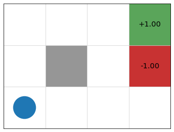
- states = cells
- actions = up, down, left, right, 10% chance of 90\(\degree\) error
- reward \(r(s) = 0\) for non-terminal nodes
- discount factor \(\gamma = 0.9\)
Value Function
A value function \(V(s)\) is a prediction of future reward attainable starting from state \(s\). \[ \begin{align} V(s) &= \max_{a \in A(s)} Q(s, a) \\ &= \max_a \mathbb{E}[R_{t+1} + \gamma R_{t+2} + \gamma^2 R_{t+3} + \ldots | S_t = s, A_t = a] \end{align} \]
Idea: lets us evaluate a state as good/bad (according to long term reward potential), and choose actions likely to take us to “better” states.
Model
A model predicts what the environment will do next
\(\mathcal{P}\) predicts the probability of the next state
\(\mathcal{R}\) predicts the expectation of the next reward, e.g.
\[ \mathcal{P}^a_{ss'} = \mathbb{P}[S_{t+1} = s' | S_t = s, A_t = a] \]
\[ \mathcal{R}^a_s = \mathbb{E}[R_{t+1} | S_t = s, A_t = a] \]
More “expensive” than learning value function or policy, which compress this info into “what I actually care about” and “what I should do”.
Categorizing RL methods
Value Based
No Policy (Implicit)
Value Function
Policy Based
Policy
No Value Function
Actor Critic
- Policy
- Value Function
Model Free
Policy and/or Value Function
No Model
Model Based
Policy and/or Value Function
Model
Value Iteration
The Bellman Equation
Value Iteration uses dynamic programming to recursively calculate a value function from an MDP.
\[ V(s) = \overbrace{\max_{a \in A(s)}}^{\text{best action from $s$}} \overbrace{\underbrace{\sum_{s' \in S}}_{\text{for every state}} P_a(s' \mid s) [\underbrace{R(s,a,s')}_{\text{(est. of) immediate reward}} + \underbrace{\gamma}_{\text{discount factor}} \cdot \underbrace{V(s')}_{\text{value of } s'}]}^{\text{expected reward $Q(s, a)$ of executing action $a$ in state $s$}} \]
Note: value iteration is model-based because it explicitly uses probability and reward distributions in calculation.
Calculating \(V(s)\) by recursion
\(V_0(s) = 0\) for all states \(s\)
\(V_{i+1}(s) = \max\limits_{a \in A(s)} \sum\limits_{s' \in S} P_a(s' \mid s) [R(s, a, s') + \gamma V_i(s')]\)
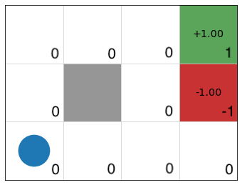
Example: GridWorld
\[ V_1(s) = \max\limits_{a \in A(s)} \sum\limits_{s' \in S} P_a(s' \mid s) R(s) + \gamma \underbrace{V_0(s')}_{0}] \]

\(V_0\)
\(V_1\)
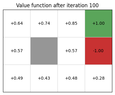
Example continued
\[ V_2(s) = \max\limits_{a \in A(s)} \sum\limits_{s' \in S} P_a(s' \mid s) [R(s) + \gamma V_1(s')] \]
\(V_1\)
\(V_2\)
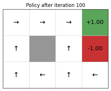
Policy Extraction
Once value function stabilizes, we extract a deterministic policy as
\[ \pi(s) = \text{argmax}_{a \in A(s)} \sum\limits_{s' \in S} P_a(s' \mid s)\ [R(s,a,s') + \gamma\ V(s')] \]
Monte Carlo Tree Search (MCTS)
Model-based methods


Replace real world with the agent’s (simulated) model of the environment
Supports rollouts (lookaheads) under imagined actions to reason about what value function will be, without further environment interaction
Model Learning
Goal: estimate model \(\mathcal{M}_\eta\) from experience \(\{S_1, A_1, R_2, \ldots, S_T\}\)
This is a supervised learning problem
\[ \begin{aligned} S_1, A_1 &\;\to\; R_2, S_2 \\ S_2, A_2 &\;\to\; R_3, S_3 \\ &\;\vdots \\ S_{T-1}, A_{T-1} &\;\to\; R_T, S_T \end{aligned} \]
Learning \(s,a \to r\) is a regression problem
Learning \(s,a \to s'\) is a density estimation problem
Pick loss function, e.g. mean-squared error, KL divergence, …
Find parameters \(\eta\) that minimise empirical loss
ExpectiMax Trees
Monte Carlo Tree search (MCTS) is based on representing MDPs as ExpectiMax trees that unfold as agents take actions.
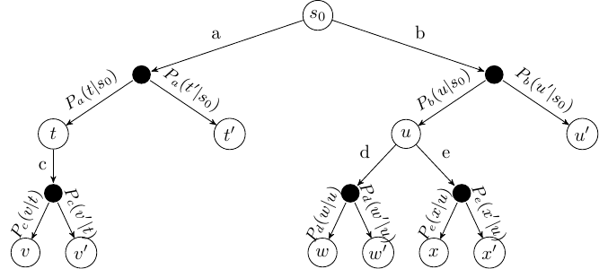
Note: state nodes are full histories
MCTS
Simultaneously “build” tree and maintain estimates of \(Q(s,a)\) by simulating trajectories and observing rewards
Focus search on promising (as indicated by \(Q\)) states when state space is too large for value iteration
Maintain visit count \(N(s)\) for states to inform strategy
MCTS Algoirithm
- Starting from root node, successively select child nodes until leaf is reached.
- Expand children by choosing action and creating new nodes based on possible outcomes.
- Simulate trajectory from one of these nodes by choosing actions either at random or with heuristic
- Backpropagate the total reward to prior nodes using Bellman equation to update \(Q(a, s)\).