07 Model-Free Prediction (Bandit Strategies + MC learning)

Slides

This module is also available in the following versions

Last Week: model-based solutions to MDPs

Value Iteration uses dynamic programming to recursively calculate a value function from an MDP.

\[ V(s) = \overbrace{\max_{a \in A(s)}}^{\text{best action from $s$}} \overbrace{\underbrace{\sum_{s' \in S}}_{\text{for every state}} P_a(s' \mid s) [\underbrace{R(s,a,s')}_{\text{immediate reward}} + \underbrace{\gamma}_{\text{discount factor}} \cdot \underbrace{V(s')}_{\text{value of } s'}]}^{\text{expected reward $Q(s, a)$ of executing action $a$ in state $s$}} \]

MCTS: simulate from forward from state $s$ and backpropagate to estimate $Q(a,s)$ for each action.

But what if you don’t have access a model/simulator?

Model-free learning

We need:

A rule for deciding which action to perform at each step based on existing knowledge —> bandit strategy
Process for aggregating & assimulating info as we go to make more informed choices in the future —> Model-free RL method, e.g. MC learning

Multi-armed Bandits

Framework for selection strategy balancing exploration and exploitation

Multi-armed bandits

Intuition: For every state $s$, each action $a$ = slot machine with initually unknown payoff distributions $X_{a}$.

The “value” $Q(s, a)$ of $a$ corresponds to (current estimate of) $X_{a}$.

\[ Q_t(a, s) = \frac{R(a, t)}{N(a,s, t)} \]

where $N(a, s, t) =$ the number of times action $a$ has been performed in state $s$ at time $t$, and $R(a, t)$ is the total reward earned from those actions as of time $t$.

Bandit algorithm

Input: Multi-armed bandit problem $M = \langle a_i \sim X_i \rangle$

Output: $Q$-values $Q(a_i)$

$Q(a_i) \leftarrow 0$ for all arms $a_i$
$N(a_i) \leftarrow 0$ for all arms $a_i$
$t \leftarrow 1$

while $t < T$ do

$a \leftarrow$ select($t$)
execute arm $a$ for round $t$ and observe reward $r(a, t)$
$N(a) \leftarrow N(a) + 1$
$Q(a) \leftarrow \left(1 - \frac{1}{N(a)}\right)Q(a) + \frac{1}{N(a)}r(a, t)$
$t \leftarrow t+1$

Bandit Selection Rules

$\epsilon$-first
$\epsilon$-greedy
$\epsilon$-decreasing
Upper confidence bound (UCB)
softmax

$\epsilon$-first

Perform random actions (explore) for $\epsilon*T$ rounds, where $T =$ total number of rounds. Then always choose $\text{argmax}_a Q(a)$ (exploit).

For each strategy, consider:

What do the parameters mean for us as modelers?
What does it mean for these numbers to be bigger/smaller?
What are the benefits and pitfalls of each strategy?
In what situations might we choose a particular strategy with particular parameter values?

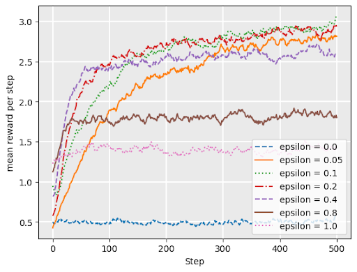
$\epsilon$-greedy

with probability $1 - \epsilon$, choose the arm with maximum $Q$-value (exploit)
with probability $\epsilon$, choose arm uniformly at random (explore)

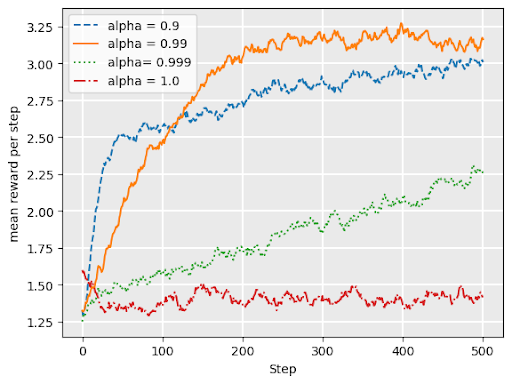
$\epsilon$-decreasing

Adds a variable $\alpha$ = “decay”
$0 < \alpha < 1$
Like $\epsilon$ greedy, but explore probability is $\epsilon*\alpha^t$ at timestep $t$
Q: what does it mean for our exploration/ exploitation strategy for $\epsilon$ to be larger (closer to 1)?

UCB1 (Upper confidence bound)

\[ \text{argmax}_{a}\Bigl( \overbrace{Q_t(a)}^{\text{exploit best action}} + \underbrace{\sqrt{\frac{2 \ln t}{N_t(a)}}}_{\text{explore to reduce ``UCB" on alternatives}}\Bigr) \]

Based on Hoeffding’s inequality in probability theory, moderates “greediness” based on the likely accuracy of estimate of $Q(a)$ given available data
UCB “exploration bonus” term grows slowly (logarithmically) with $t$, but shrinks with larger sample size $N_t(a)$.

softmax

\[ P(a) = \frac{e^{Q(a)/\tau}}{\sum_{b\in A} e^{Q(b)/\tau}} \]

Approximates ratio of (exponential function of) current expected return for $a$ compared to alternatives

$\tau$ $\geq 0$ is the temperature parameter. Dictates influence of current value of $Q$ on decision.

lower $\tau$ = more exploitation: small differences in $Q$ get amplified in exponent, approaching argmax as $\tau \to 0^+$.
higher $\tau$ = more exploration: approaches uniform random as $\tau \to \infty$.

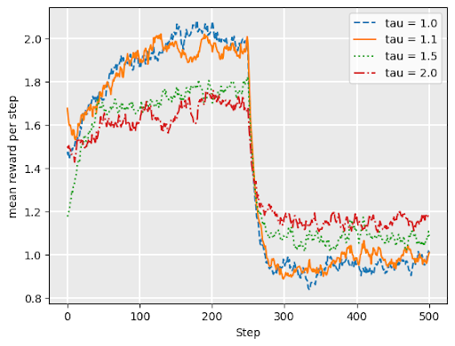
softmax continued

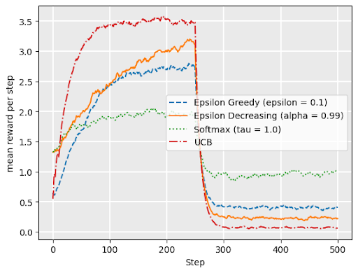
Softmax works well under drift– when underlying reward distributons change over time
Graph shows softmax performance for “restless bandit” where reward distributions abruptly change at $t= 250$.

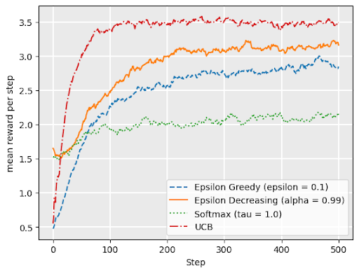
Comparing bandit strategies

no drift

drift

Upper Confidence Trees (UCT)

MCTS commonly uses a variant of UCB for its selection rule:

\[ \text{argmax}_{a \in A(s)} \Bigl( Q(s, a) + \alpha\sqrt{\frac{2 \ln(N(s))}{N(s, a)}} \Bigr) \]

where $N(s)$ is the number of times a node has been visited, $N(s, a)$ is the number of times action $a$ has been chosen in that state, and $\alpha$ is an exploration parameter.

Note: when $N(a) = 0$, second term is “infinity”, i.e., always choose unexplored actions first.

Monte Carlo Learning

Estimating Q(a,s) from experience

Idea:

Each state $s$ viewed as bandit problem with arms $A(s)$
The “payoff” for each “arm” $a$ is given by the total discounted reward $G$ collected during an episode which starts by performing action $a$ in state $s$ \[ \begin{align} G_t &= r(s_t, a_t, s_{t+1}) + \gamma r(s_{t+1}, a_{t+1}, s_{t_2}) + \gamma^2... \\ &= r(s_t, a_t, s_{t+1}) + \gamma G_{t+1} \end{align} \]
Maintain Q-function data structure that updates estimate $Q(s,a)$ after each episode to reflect average return $G$

Q-tables

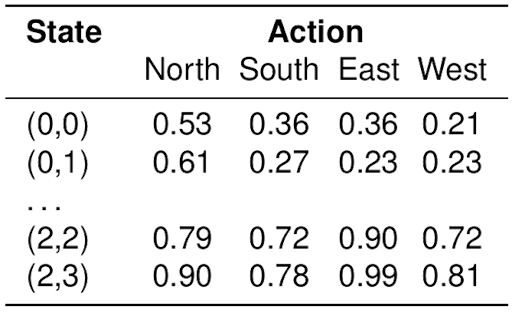
$Q(s, a)$ indicates our current guess (observed average) for the long term expected discounted reward associated with taking action $a$ in state $s$

MC learning algorithm

Initialize $Q(s, a) \leftarrow 0$
Generate episode using bandit strategy:

\[ s_0, a_0, r_0, s_1, a_1, r_1, s_2, a_2, ... s_T, a_T, r_T \]

initialize discounted future reward for episode $G \leftarrow 0$
Working back to front for each (first appearance of) pair $(s_t, a_t)$, update $G$ and $Q$ as

\[ \begin{align} G &\leftarrow r_t + \gamma G \\ Q(s_t, a_t) &\leftarrow \left( 1 - \frac{1}{N(s_t, a_t)} \right) Q(s_t, a_t) + \frac{1}{N(s_t, a_t)} G \end{align} \]

Repeat until $Q$ converges (or time/resource budget used up)

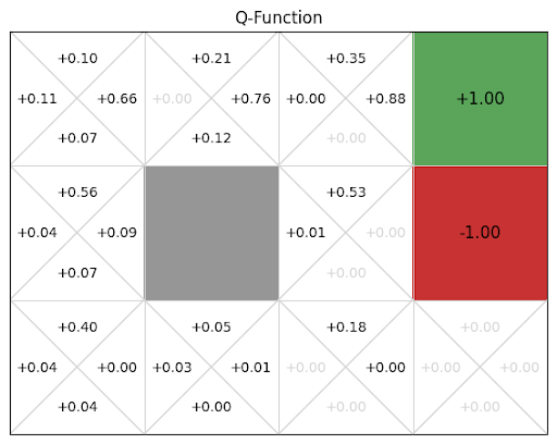
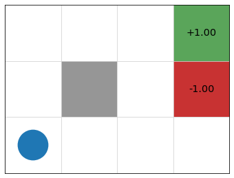
Gridworld Example

Update $Q$-table (initialized to 0) based on this trajectory:

$s_0 = (1, 1)$, $a_0 =$ up, $r_0 = 0$,

$s_1 = (2, 1)$, $a_1 =$ right, $r_1 = 0$,

$s_2 = (3, 1)$, $a_2 =$ up, $r_2 = 0$,

$s_3 = (3, 2)$, $a_3 =$ up, $r_3 = 0$,

$s_4 = (4, 2)$, $a_4 =$ claim reward, $r_4 = -1$.