09 Value Function Approximation (Deep RL)
Slides
This module is also available in the following versions
Value Function Approximation
So far we have represented value function by a lookup table
Every state \(s\) has an entry \(V(s)\),
or every state-action pair \((s,a)\) has an entry \(Q(s,a)\)
Problem with large MDPs
Too many states and/or actions to store in memory
Too slow to learn the value of each state individually
Solution for large MDPs
Estimate value function with function approximation
\[\begin{align*} \hat{V}(s; {\color{red}{\mathbf{w}}})\; & {\color{blue}{\approx}}\; V_{\pi}(s)\\[0pt] \text{or}\;\;\;\hat{Q}(s, a; {\color{red}{\mathbf{w}}})\; & {\color{blue}{\approx}}\; Q_{\pi}(s, a) \end{align*}\]
Generalises from seen states to unseen states
- Parametric function approximation to the true value function, \(V_{\pi}(s)\) or action-value function \(Q_{\pi}(s,a)\)
Update parameter \({\color{red}{\mathbf{w}}}\) (a vector) using MC or TD learning
- Less memory required, based only on number of weights in vector \({\color{red}{\textbf{w}}}\), instead of number of states \(s\) (\(s\) becomes implicit)
Example: Frogger
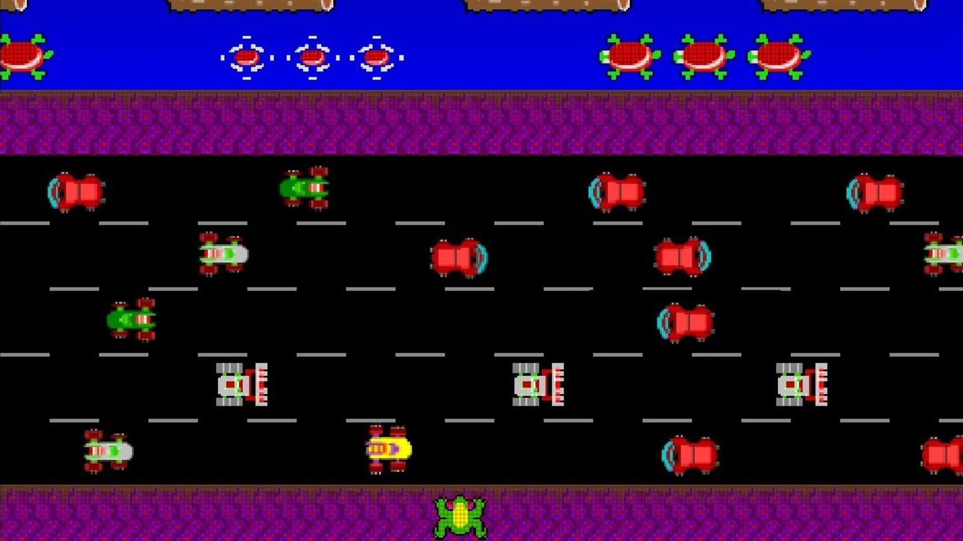
States: coords of frog & cars,
Actions: stay or move frog up, down, left right
All top row states are terminal with + reward. Frog getting hit by car also terminal, (0 or negative reward.)
Question: What “features” of states are most relevant for determining value function \(V(s)\)?
Feature Vectors
Represent state by a feature vector
\[ \mathbf{x}(s) = \begin{pmatrix} x_1(s) \\ \vdots \\ x_n(s) \end{pmatrix} \]
In Frogger example:
- Vertical distance of frog from top row
- Horizontal distance of cars in current row, row above, and row below
- Maybe: color or orientation of vehicles
Linear Value Function Approximation
Represent value function by a linear combination (weighted sum) of features:
\[
\hat{V}(s; \mathbf{w}) = \mathbf{x}(s)^\top \mathbf{w} = \sum_{j=1}^n x_j(s) w_j
\]
During TD or MC learning, updates weights rather than \(Q(s,a)\) or \(V(s)\), directly, i.e.
\[ w^a_i \leftarrow w^a_i + \alpha \cdot \delta \cdot \ x_i(s, a) \]
Where \(\delta\) is the TD error [new TD estimate]- [prior \(Q(a, s)\) or \(V(s)\)]
This implicitly updates value function for all states in accordance with value function representation.
Defining State-Action Features
Since it may be easier to define features for states rather than state/action pairs, we can extend state features \(x_i\) to state action pairs as
\[ \begin{split} x_{i,k}(s,a) = \Bigg \{ \begin{array}{ll} x_i(s) & \text{if } a=a_k\\ 0 & \text{otherwise} \end{array} \end{split} \]
If we had \(n\) state features before, we know have \(n*|A|\). This effectively gives us \(|A|\) different weight vectors, one for each action, since the linear representation of \(Q(s, a_k)\) only has non-zero components for \(x_{i, k}\):
\[ \hat{Q}(s, a_k; \mathbf{w}) = \sum\limits_{i = 1, j = 1}^{i = n, j = |A|}w_{i}^j \cdot x_{i, k}(s, a_j) = \sum\limits_{i = 1}^n w^{k}_i x_i(s) \]
Example: Frogger Linear Approximation + SARSA
\(x_0 \equiv 1\) bias term (learns default value of states/actions in absence of features)
\(x_ 1 = x_{\text{dist}} = \frac{\text{current row}}{\text{total rows}}\), i.e. normalized vertical distance.
\(x_2, x_3, x_4 = x_{\text{current}}, x_{\text{above}}, x_{\text{below}} =\) (normalized) horizontal distance from nearest car in current row, row above, and row below.
Initialize \(w_{\text{feature}}^{\text{action}} = 0\) for all features and actions.
At each time step, bandit strategy to select action \(a\), observe reward \(r\) and state \(s'\), and select next action \(a'\).
Calculate temporal difference
\[ \delta = r + \gamma \hat{Q}(s', a'; \mathbf{w}) - \hat{Q}(s, a; \mathbf{w}) = r + \gamma \sum_{i=0}^4 w_i^{a'}x_i(s') - \sum_{i=0}^4 w_i^{a}x_i(s) \]
For each feature \(x_i\), update weight \(w_{i}^{a}\) as \(w_{i}^{a} \leftarrow w_{i}^{a} + \alpha \cdot \delta \cdot x_i(s)\).
Generalizing to non-linear approximation
With TD learning, we are trying make \(\hat Q(s, a, \mathbf{w})\) closer to our TD target \(r + \gamma \hat{V}(s',\mathbf{w})\) by adjusting the weights \(w_i\). We can express this in terms of trying to minimize a squared Bellman error loss function:
\[ L(\mathbf{w}) = \frac{1}{2}(\text{target} - \text{prediction})^2 = \frac{1}{2} (r + \gamma \hat{V}(s',\mathbf{w}) - \hat Q(s, a; \mathbf{w}))^2 \]
The update rule we chose is equivalent to performing semi-gradient descent on \(L\). Its semi-gradient in the sense that we are treating the TD target as fixed. We minimize this loss function by adjusting the weights \(\mathbf{w}\) in the direction of the negative gradient of \(L\), i.e.
\[ w_i \leftarrow w_i - \alpha \frac{\partial L(\mathbf{w})}{\partial w_i} = w_i + \alpha \delta \frac{\partial \hat Q(s, a; \mathbf{w})}{\partial w_i} = w_i + \alpha \delta x_i(s, a) \]
This last equality only holds in the linear case, where changing \(w_i \to w_i + \Delta\) changes \(Q\) by \(+ \Delta x_i\)
Gradient Descent
Let \(J(\mathbf{w})\) be a differentiable objective function of parameter vector \(\mathbf{w}\)
Define the gradient of \(J(\mathbf{w})\) to be
\[
{\color{red}{\nabla_{\textbf{w}} J(\mathbf{w})}} =
\begin{pmatrix}
\frac{\partial J(\mathbf{w})}{\partial \mathbf{w}_1} \\
\vdots \\
\frac{\partial J(\mathbf{w})}{\partial \mathbf{w}_n}
\end{pmatrix}
\]
To find a local minimum of \(J(\mathbf{w})\)
Adjust \(\mathbf{w}\) in direction of negative gradient
\(\;\;\;\;\;\;\Delta \mathbf{w} = -\alpha \nabla_{\mathbf{w}} J(\mathbf{\mathbf{w}})\)
i.e. move downhill (\(\nabla\) is differential operator for vectors and \(\alpha\) is a step-size parameter)

Deep Q-function Approximation
The general expression for the update rule,
\[ \theta \leftarrow \theta + \alpha \cdot \delta \cdot \nabla_{\theta} \hat Q(s,a; \theta) \]
lets us take advantage of deep learning methods for learning a function estimate \(Q(s,a) \approx \hat Q(s,a; \theta)\) parameterised by weights \(\theta\) in a deep neural network.
With linear approximation, \(\nabla_{\mathbf{w}} \hat Q(s,a; \mathbf{w}) = \mathbf{x}(s, a)\). For complex non-linear functions, it’s harder to compute the gradient.
Backpropagating through the neural network effectively computes this for us. It sends the error signal from the TD estimate back through the network to adjust weights in order to reduce that error.
Deep SARSA for Frogger
Define a neural network that takes state action pairs as inputs and outputs a prediction \(\hat Q(s,a; \theta)\) for \(Q(s, a)\). Initialize parameters \(\theta\) arbitrarily.
Proceed as with linear TD approximation, using \(\hat Q_\theta\) + bandit method to select action, observe reward and state, and pick next action. Compute temporal difference
\[ \delta = r + \gamma \hat Q(s',a'; \theta) - \hat Q(s,a; \theta) \]
Backpropagate the loss (\(L(\theta) = \frac{1}{2} \delta^2\)) through the network to adjust neural network weights \(\theta\) to move \(\hat Q(s,a; \theta)\) closer to target SARSA target \(r + \gamma \hat Q(s',a'; \theta)\), treating target as fixed.