9 Model-Free Prediction & Control (MC and TD Learning, Sarsa and Q-Learning)
Slides
This module is also available in the following versions
Model-Free Reinforcement Learning
Last Module (8):
Integrating learning and planning
Use planning to construct a value function or policy
This Module (9):
Model-free prediction and control
Prediction: Optimise the value function of an unknown MDP
Control: Learn model directly from experience
Monte-Carlo Learning
Monte-Carlo Reinforcement Learning
MC methods learn directly from episodes of experience
- MC is model-free: no knowledge of MDP transitions / rewards
MC learns from complete episodes
- No bootstrapping, as we will see later
MC uses the simplest possible idea of looking at sample returns: value = mean return
- Caveat: can only apply to episodic MDPs, i.e. all episodes must terminate
Monte-Carlo Policy Evaluation
- Goal: learn \(v_\pi\) from episodes of experience under policy \(\pi\)
\[ S_1, A_1, R_2, \ldots, S_k \sim \pi \]
- Recall that the return is the total discounted reward:
\[ G_t = R_{t+1} + \gamma R_{t+2} + \ldots + \gamma^{T-1} R_T \]
- Recall that the value function is the expected return:
\[ v_\pi(s) = \mathbb{E}_\pi \left[ G_t \mid S_t = s \right] \]
Monte-Carlo policy evaluation uses empirical mean return instead of expected return
Computes empirical mean from the point \(t\) onwards using as many samples as we can
Will be different for every time step
First-Visit Monte-Carlo Policy Evaluation
To evaluate state, \(s\):
- On the first time-step, \(t\) that state, \(s\), is visited in an episode:
- Increment counter \(N(s) \leftarrow N(s) + 1\)
- Increment total return \(S(s) \leftarrow S(s) + G_t\)
- Estimate: \[ V(s) = \frac{S(s)}{N(s)} \]
By Law of Large Numbers, \(V(s) \to v_\pi(s)\) as \(N(s) \to \infty\)
- Only requirement is we somehow visit all of these states
The Central Limit Theorem tells us how quickly it approaches the mean
The variance (mean squared error) of estimator reduces with \(\frac{1}{N}\)
i.e. rate is independent of size of state space, \(|\mathcal{s}|\)
speed depends on how many episodes/visits reach \(s\) (coverage probabilities).
Every-Visit Monte-Carlo Policy Evaluation
To evaluate state, \(s\):
- Every time-step, \(t\), that state, \(s\), is visited in an episode:
- Increment counter \(N(s) \leftarrow N(s) + 1\)
- Increment total return \(S(s) \leftarrow S(s) + G_t\)
- Increment counter \(N(s) \leftarrow N(s) + 1\)
- Estimate:
\[ V(s) = \frac{S(s)}{N(s)} \]
Again, \(V(s) \to v_\pi(s)\) as \(N(s) \to \infty\).
First-Visit versus Every-Visit Monte-Carlo Policy Evaluation?
Every-Visit Advantages:
Especially good when episodes are short or when states are rarely visited — no sample gets “wasted.”
i.e. uses more of the data collected, often faster convergence in practice.
First-visit Advantages:
Useful when episodes are long and states repeated many times.
i.e. avoids dependence between multiple visits to the same state in one episode.
Blackjack Example
States (\(\sim 200\)):
Current sum of cards (\(12-21\))
Dealer’s showing card (Ace\(-10\))
Whether you have a usable ace - (can be counted as \(1\) or \(11\) without busting \(>21\)) (yes/no)
Actions:
Stand: stop receiving cards (and terminate)
Hit: take another card (no replacement)
Transitions:
- You are automatically hit if your sum \(< 12\)
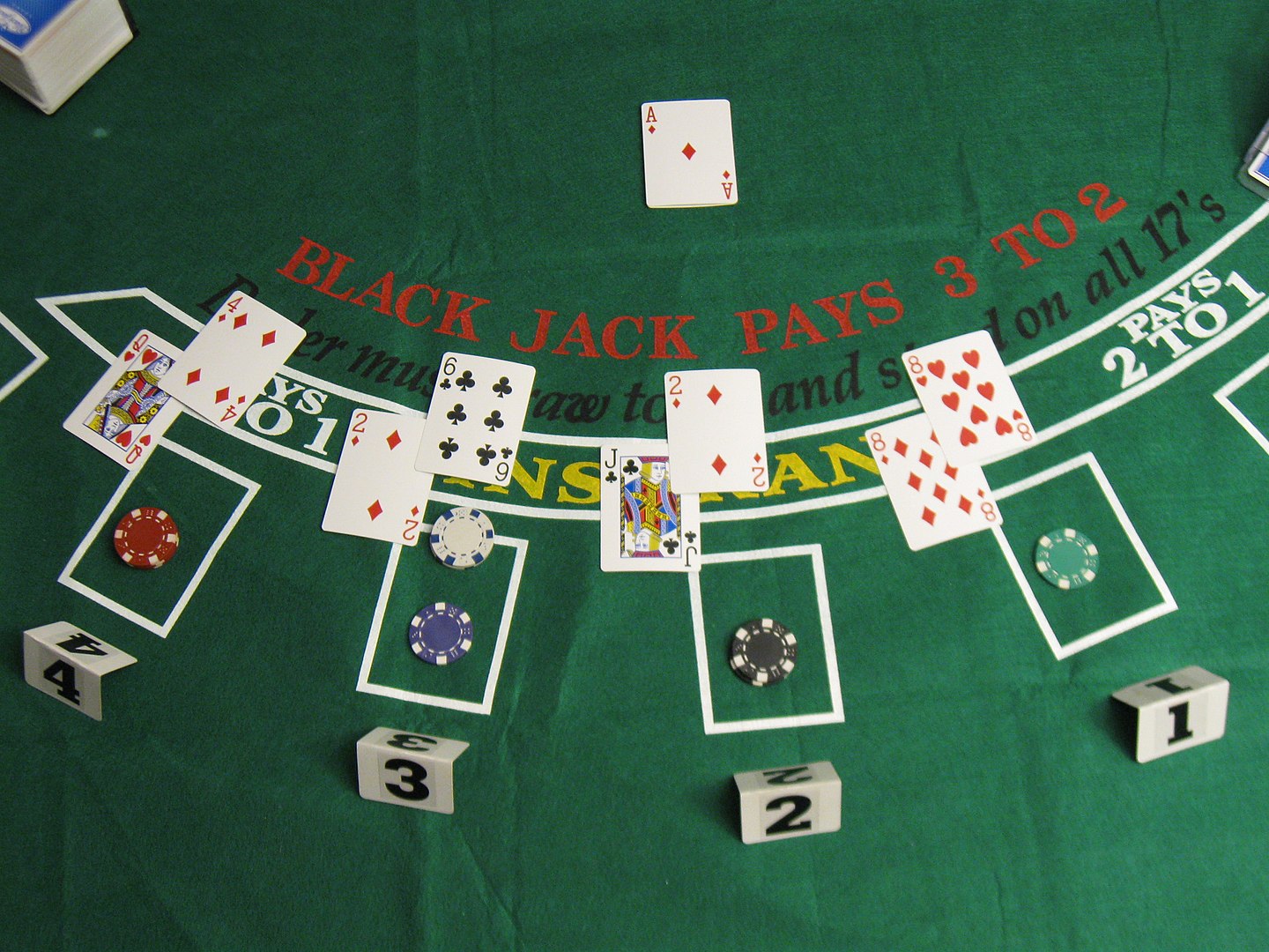
Rewards:
For stand: \(+1\) if your sum \(>\) dealer’s; \(0\) if equal; \(−1\) if less
For hit: \(−1\) if your sum \(> 21\) (and terminate); \(0\) otherwise
Blackjack Value Function after Monte-Carlo Learning

Policy: stand if sum of cards ≥ 20, otherwise hit
Learning value function directly from experience
Usable ace value is noisier because the state is rarer
Key point: once we have learned the value function from experience,
- we can evaluate actions for making the best decision for optimising a policy as we will see later
Incremental Mean (Refresher)
The mean \(\mu_1, \mu_2, \cdots\) of a sequence \(x_1, x_2, \dots\) can be computed incrementally,
\[\begin{align*} \mu_k & = \frac{1}{k} \sum_{j=1}^k x_j\\[2pt] & = \frac{1}{k}\left(x_k + \sum_{j=1}^{k-1} x_j\right)\\[2pt] & = \frac{1}{k}(x_k + (k - 1) \mu_{k-1})\\[2pt] & = \mu_{k-1} + \frac{1}{k}({\color{red}{x_k - \mu_{k-1}}}) \end{align*}\]
\({\color{red}{\mu_{k-1}}}\) is the previous mean: predicts what think value will be
\({{\color{red}{x_k}}}\) is the new value
Incrementally corrects mean \(\frac{1}{k}\) in direction of error \({\color{red}{x_k - \mu_{k-1}}}\)
Incremental Monte-Carlo Updates (Same idea)
Update \(V(s)\) incrementally after each episode \(S_1, A_1, R_2, \dots, S_T\):
- For each state \(S_t\) with return \(G_t\):
\[ \begin{aligned} N(S_t) &\leftarrow N(S_t) + 1 \\ V(S_t) &\leftarrow V(S_t) + \frac{1}{N(S_t)}\,({\color{red}{G_t - V(S_t)}}) \end{aligned} \]
In non-stationary problems, it can be useful to track a running mean by forgetting old episodes using a constant step size \(\alpha\):
\[ V(S_t) \leftarrow V(S_t) + \alpha ( G_t - V(S_t) ) \]
A constant step size turns the MC estimate into an exponentially weighted moving average of past returns
- Decays geometrically with visits - the return from \(k\) visits ago depends on \(\alpha(1 - \alpha)^k\)), instead of arithmetically according to \(N\) returns having an equal weight of \(\frac{1}{N}\)
In general, we prefer non-stationary estimators because our policy we will be evaluating is continuously improving
- Essentially we are always in a non-stationary setting in RL as we improve our policy through experience
In summary, in Monte-Carlo learning we
- Run out episodes,
- look at the complete returns, and
- update estimates of the mean value of return at each state of the return.
Temporal-Difference Learning
Temporal-Difference (TD) Learning
TD methods learn directly from episodes of experience
- TD is model-free: no knowledge of transitions/rewards (as in MC)
TD learns from incomplete episodes, by bootstrapping
It substitutes, or bootstraps, reminder of the trajectory with the estimate of what will happen, instead of waiting for full returns
i.e. TD updates one guess with a subsequent guess
MC versus TD
Goal: learn \(v_\pi\) online from experience under policy \(\pi\)
Incremental every-visit Monte-Carlo:
Update value \(V(S_t)\) toward actual return \({\color{red}{G_t}}\)
\[ V(S_t) \leftarrow V(S_t) + \alpha \left({\color{red}{G_t}}- V(S_t) \right) \]
Simplest temporal-difference learning algorithm: TD(0):
Update value \(V(S_t)\) toward estimated return \({\color{red}{R_{t+1} + \gamma V (S_{t+1})}}\) (like Bellman equation)
\[ V(S_t) \leftarrow V(S_t) + \alpha \left({\color{red}{R_{t+1} + \gamma V(S_{t+1})}} - V(S_t) \right) \]
\(R_{t+1} + \gamma V(S_{t+1})\) is called the TD target (we are moving towards) \(\delta_t = R_{t+1} + \gamma V(S_{t+1}) - V(S_t)\) is called the TD error
Driving Home Example
| State | Elapsed Time (min) | Predicted Time to Go | Predicted Total Time |
|---|---|---|---|
| leaving office | 0 | 30 | 30 |
| reach car, raining | 5 | 35 | 40 |
| exit highway | 20 | 15 | 35 |
| behind truck | 30 | 10 | 40 |
| home street | 40 | 3 | 43 |
| arrive home | 43 | 0 | 43 |
Driving Home Example: MC versus TD
Changes recommended by Monte Carlo methods \((\alpha=1)\):
Changes recommended by TD methods \((\alpha=1)\):

Red arrow represent recommended updates by MC and TD respectively
Advantages & Disadvantages of MC versus TD
TD can learn before knowing the final outcome
- TD can learn online after every step
- MC must wait until end of episode before return is known
TD can learn without the final outcome
- TD can learn from incomplete sequences
- MC can only learn from complete sequences
- TD works in continuing (non-terminating) environments
- MC only works for episodic (terminating) environments
Bias/Variance Trade-Off
Return \(G_t = R_{t+1} + \gamma R_{t+2} + \dots + \gamma^{T-1} R_T\) is an unbiased estimate of \(v_\pi(S_t)\).
True TD target \(R_{t+1} + {\color{blue}{\gamma\, v_\pi(S_{t+1}}})\) is an unbiased estimate of \(v_\pi(S_t)\).
TD target \(R_{t+1} + \gamma\, V(S_{t+1})\) is a biased estimate of \(v_\pi(S_t)\).
TD target has much lower variance than the return, since
Return depends on many random actions, transitions, rewards.
TD target depends on one random action, transition, reward.
Advantages & Disadvantages of MC versus TD (2)
MC has high variance, zero bias
Good convergence properties (even with function approximation)
Not very sensitive to initial value
Very simple to understand and use
TD has low variance, some bias
Usually more efficient than MC
TD(0) converges to \(v_{\pi}(s)\) (but not always with function approximation)
More sensitive to initial value
Random Walk Example


Random Walk example based on uniform random policy: left 0.5 and right 0.5
Random Walk: MC versus TD

- This demonstrates the benefit of bootstrapping
Batch MC and TD
MC and TD both converge in the limit
- \(V(s) \to v_{\pi}(s)\) as experience \(\rightarrow \infty\)
What about a batch solution for finite experience, \(k\) finite episodes?
\[ s^1_1, a^1_1, r^1_2, \cdots s^1_{T_1} \]
\[ \vdots \]
\[ s^K_1, a^K_1, r^K_2, \cdots s^K_{T_K} \]
In batch mode you repeatedly sample episode \(k \in [1, K]\) and apply MC or TD(0) to episode \(k\)
AB Example
Two states \(A, B\); no discounting; 8 episodes:
\(A, 0, B, 0\)
\(B, 1\)
\(B, 1\)
\(B, 1\)
\(B, 1\)
\(B, 1\)
\(B, 1\)
\(B, 0\)

Clearly, \(V(B)\) = \(\frac{6}{8} = 0.75\), but what about \(V(A)\)?
Certainty Equivalence
MC converges to solution with minimum mean-squared error
- Best fit to the observed returns
\[ \sum_{k=1}^K \sum_{t=1}^{T_k} \left( G_t^k - V(s_t^k) \right)^2 \]
- In the AB example, \(V(A) = 0\)
TD(\(0\)) converges to solution of max likelihood Markov model that best explains the data
- Solution to the MDP \(\langle \mathcal{S}, \mathcal{A}, \hat{\mathcal{P}}, \hat{\mathcal{R}}, \gamma \rangle\) that best fits the data (\(\hat{\mathcal{P}}\) counts the transitions, and \(\hat{\mathcal{R}}\) the rewards)
\[ \hat{\mathcal{P}}_{s,s'}^a \;=\; \frac{1}{N(s,a)} \sum_{k=1}^K \sum_{t=1}^{T_k} \mathbf{1}\!\left( s_t^k, a_t^k, s_{t+1}^k = s, a, s' \right) \]
\[ \hat{\mathcal{R}}_s^a \;=\; \frac{1}{N(s,a)} \sum_{k=1}^K \sum_{t=1}^{T_k} \mathbf{1}\!\left( s_t^k, a_t^k = s, a \right) r_t^k \]
- In the AB example, \(V(A) = 0.75\)
Advantages and Disadvantages of MC versus TD (3)
TD exploits Markov property
- Usually more efficient in Markov environments
MC does not exploit Markov property
Usually more effective in non-Markov environments
Note that partial observability and non-stationarity are reasons an environment can be non-Markov
Monte-Carlo Backup
\[ V(S_t) \;\leftarrow\; V(S_t) + \alpha \big( G_t - V(S_t) \big) \]

Starting at one state, sample one complete trajectory to update the value function
Temporal-Difference Backup
\[ V(S_t) \;\leftarrow\; V(S_t) + \alpha \big( R_{t+1} + \gamma V(S_{t+1}) - V(S_t) \big) \]

In TD backup is just over one step
Tree Search/Dynamic Programming Backup
\[ V(S_t) \;\leftarrow\; \mathbb{E}_\pi \!\left[ R_{t+1} + \gamma V(S_{t+1}) \right] \]

If we know the dynamics of the environment, we can do search and a complete backup over the tree
Bootstrapping and Sampling
Bootstrapping: update involves an estimate
MC does not bootstrap
Tree Search (with heuristic search) or dynamic programming bootstraps
TD bootstraps
Sampling: update samples an expectation
MC samples
Tree Search does not sample
TD samples
Unified View of Reinforcement Learning (1)

Unified View of Reinforcement Learning (2)

Dynamic programming only explores one level, in it’s most simple form.
In practice, dynamic programming is used during tree search, similar to classical planning.
TD(λ)
\(n\)-Step Prediction
Let TD target look \(n\) steps into the future

\(n\)-Step Return
Consider the following \(n\)-step returns for \(n=1, 2, \infty\): \[\begin{align*} \color{red}{n} & \color{red}{= 1}\ \text{(TD(0))} & G_t^{(1)} & = R_{t+1} + \gamma V(S_{t+1})\\[2pt] \color{red}{n} & \color{red}{= 2} & G_t^{(2)} & = R_{t+1} + \gamma R_{t+2} + \gamma^2 V(S_{t+2})\\[2pt] \color{red}{\vdots} & & \vdots & \\[2pt] \color{red}{n} & \color{red}{= \infty}\ \text{(MC)} & G_t^{(\infty)} & = R_{t+1} + \gamma R_{t+2} + \cdots + \gamma^{T-1} R_T \end{align*}\]
Define the \(n\)-step Return (real reward \(+\) estimated reward, \({\color{blue}{\gamma^n V(S_{t+n})}}\)):
\[ G^{(n)}_t = R_{t+1} + \gamma R_{t+2} + \cdots + \gamma^{n-1} R_{t+n} + {\color{blue}{\gamma^n V(S_{t+n})}} \]
\(n\)-step temporal-difference learning (updated in direction of error)
\[ V(S_t) \;\leftarrow\; V(S_t) + \alpha \big({\color{red}{G_t^{(n)} - V(S_t)}} \big) \]
MC looks at the real reward
So which \(n\) is the best?
Large Random Walk Example

- RMS errors vary according to step size \(\alpha\), with the optimum dependent on \(n\)
Note that RMS errors also vary according to whether learning is on-line or off-line updates (not shown here)
- i.e. whether immediately update value function or defer updates until episode ends
Averaging \(n\)-Step Returns
We can form mixtures of different \(n\):
e.g. average of \(2\)-step and \(4\)-step returns:
\[ \frac{1}{2} G_t^{(2)} + \frac{1}{2} G_t^{(4)} \]
We can average \(n\)-step returns over different n
- e.g. average the 2-step and 4-step returns
Combines information from two different time-steps
Can we efficiently combine information from all time-steps to be more robust?

\(\lambda\)-return

The \(\lambda\)-return \(G_t^{\lambda}\) combines all \(n\)-step returns \(G_t^{(n)}\)
- Using weight \({\color{red}{(1 - \lambda)\lambda^{\,n-1}}}\)
\[ G_t^{\lambda} \;=\; {\color{red}{(1 - \lambda) \sum_{n=1}^{\infty} \lambda^{\,n-1}}} G_t^{(n)} \]
Forward-view TD(\(\lambda\))
\[ V(S_t) \;\leftarrow\; V(S_t) + \alpha \big( G_t^{\lambda} - V(S_t) \big) \]
TD(\(\lambda\)) Weighting Function

\[ G_t^{\lambda} \;=\; (1 - \lambda) \sum_{n=1}^{\infty} \lambda^{\,n-1} G_t^{(n)} \]
- \(\lambda\)-return is a geometrically weighted return for every \(n\)-step return
Note that geometric weightings are memoryless
- i.e. we can compute \(TD(\lambda)\) with with no greater complexity than \(TD(0)\)
However, the formulation presented so far is a forward view
- we can’t look into the future!
Forward View of TD(λ)

Update value function towards the \(\lambda\)-return
Forward-view looks into the future to compute \(G^{\lambda}_t\)
Like MC, can only be computed from complete episodes
We will see shortly how an iterative algorithm achieves the forward view without having to wait until the future
Forward View of TD(λ) on Large Random Walk

We can see using TD(\(\lambda\)), and choosing \(\lambda\) value (left hand side), is more robust than choosing a unique \(n\)-step value (right hand side)
- \(\lambda=1\) is MC and \(\lambda=0\) is TD(\(0\))
Backward View of TD(\(\lambda\))
Forward view provides theory
Backward view provides mechanism
Update online, every step, from incomplete sequences
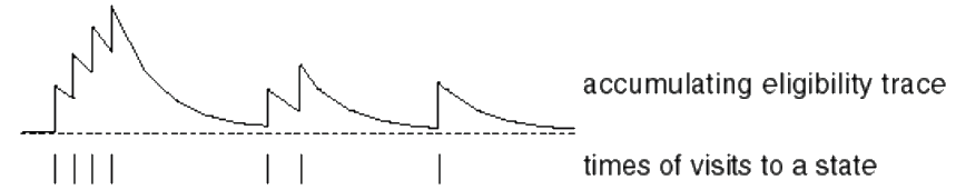
Eligibility Traces

Credit assignment problem: did bell or light cause shock?
Frequency heuristic: assign credit to most frequent states
Regency heuristic: assign credit to most recent states
Eligibility traces combine both heuristics
\[\begin{align*} E_0(s) & = 0\\[2pt] E_t(s) & = \gamma \lambda E_{t-1}(s) + 1(S_t = s) \end{align*}\]
Backward View TD(\(\lambda\))
Keep an eligibility trace for every state \(s\)
Update value \(V(s)\) for every state \(s\)
In proportion to TD-error \(\delta_t\) and eligibility trace \(E_t(s)\)
\[ \delta_t = R_{t+1} + \gamma V(S_{t+1}) - V(S_t) \]
\[ V(s) \;\leftarrow\; V(s) + \alpha \,\delta_t E_t(s) \]

TD(\(\lambda\)) and TD(\(0\))
When \(\lambda = 0\), only the current state is updated.
\[E_t(s) = \mathbf{1}(S_t = s)\] \[V(s) \leftarrow V(s) + \alpha\,\delta_t\,E_t(s)\]
This is exactly equivalent to the TD(\(0\)) update.
\[V(S_t) \leftarrow V(S_t) + \alpha\,\delta_t\]
TD(\(\lambda\)) and MC
When \(\lambda = 1\), credit is deferred until the end of the episode.
- Consider episodic environments with offline updates.
- Over the course of an episode, the total update for TD(\(\lambda\)) is the same as the total update for MC.
Theorem
The sum of offline updates is identical for forward-view and backward-view TD(\(\lambda\)):
\[ \sum_{t=1}^{T} \alpha\,\delta_t\,E_t(s) \;=\; \sum_{t=1}^{T} \alpha \bigl( G_t^{\lambda} - V(S_t) \bigr)\,\mathbf{1}(S_t = s). \]
Example: Temporal-Difference Search for MCTS
Example: Temporal-Difference Search for MCTS
Simulation-based search
\(\ldots\) using TD instead of MC (bootstrapping)
MC tree search applies MC control to sub-MDP from now
TD search applies Sarsa to sub-MDP from now
MC versus TD search
For model-free reinforcement learning, bootstrapping is helpful
TD learning reduces variance but increases bias
TD learning is usually more efficient than MC
TD(\(\lambda\)) can be much more efficient than MC
For simulation-based search, bootstrapping is also helpful
TD search reduces variance but increases bias
TD search is usually more efficient than MC search
TD(\(\lambda\)) search can be much more efficient than MC search
TD search
Simulate episodes from the current (real) state \(s_t\)
Estimate action-value function \(Q(s,a)\)
- For each step of simulation, update action-values by Sarsa
\[ \Delta Q(S,A) = \alpha \big( R + \gamma Q(S',A') - Q(S,A) \big) \]
- Select actions based on action-values \(Q(s,a)\)
- e.g. \(\epsilon\)-greedy
May also use function approximation for \(Q\), if needed
Results of TD search in Go
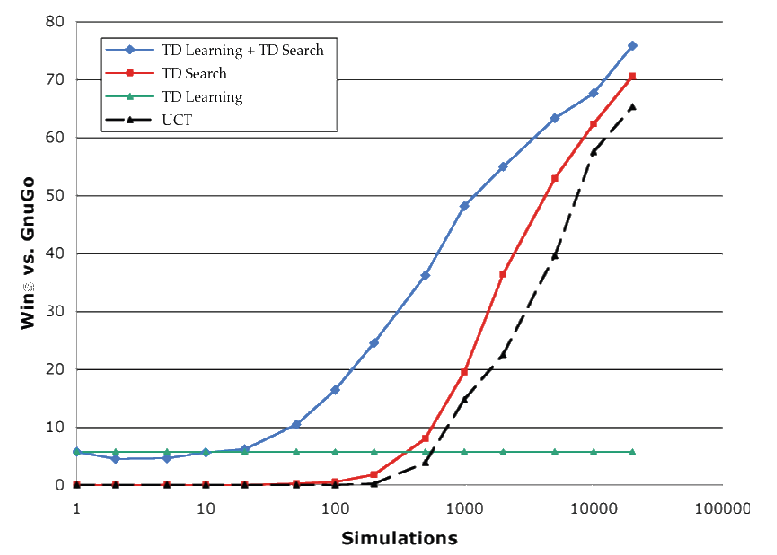
Black dashed line is MCTS
Blu line is Dyna-Q (not covered in this module)
Learning from simulation is an effective method in search
Model-Free Control (Sarsa and Q-Learning)
Uses of Model-Free Control
Example problems that can be naturally modelled as MDPs
- Elevator
- Parallel Parking
- Ship Steering
- Bioreactors
- Power stations
- Computer Programming
- Fine tuning LLMs
- Portfolio management
- Protein Folding
- Robot walking
For most of these problems, either:
- MDP model is unknown, but experience can be sampled
- MDP model is known, but is too big to use, except by samples
Model-free control can solve these problems
On and Off-Policy Learning
On-policy learning
“Learn on the job”
Learn about policy \(\pi\) from experience sampled from \(\pi\)
Off-policy learning
“Look over someone’s shoulder”
Learn about policy \(\pi\) from experience sampled from \({\color{red}{\mu}}\)
Off-policy learning uses trajectories sampled from policy \({\color{red}{\mu}}\), e.g. from another robot, AI agent, human, or simulator.
On-Policy Monte-Carlo Control
Generalised Policy Iteration

Alternation converges on optimal policy \(\pi_\ast\)
Policy evaluation Estimate \(v_{\pi}\)
e.g. Iterative policy evaluation, going upPolicy improvement Generate \(\pi^{\prime} \geq \pi\) e.g. Greedy policy improvement, act greedily with respect to value function, going down

Principle of Optimality
Any optimal policy can be subdivided into two components:
An optimal first action \(A_*\)
Followed by an optimal policy from successor state \(S'\)
Generalised Policy Iteration with Monte-Carlo Evaluation
Policy evaluation 1. Can we use Monte-Carlo policy evaluation to estimate \({\color{blue}{V = v_{\pi}}}\)(running multiple episodes/rollouts)?
Policy improvement 2. Can we do greedy policy improvement with MC evaluation?
Model-Free Policy Iteration Using Action-Value Function
- Problem 1: Greedy policy improvement over \(V(s)\) requires a model of MDP
\[ \pi'(s) \;=\; \arg\max_{a \in \mathcal{A}} \Big[ \mathcal{R}^a_s \;+\; {\color{red}{\sum_{s'} P^a_{ss'} \, V(s')}} \Big] \]
- Alternative: use action-value functions in place of model Greedy policy improvement over \(Q(s,a)\) is model-free
\[ \pi'(s) \;=\; \arg\max_{a \in \mathcal{A}} Q(s,a) \]
Generalised Policy Iteration with Action-Value Function

Policy evaluation We run Monte-Carlo policy evaluation using \({\color{red}{Q=q_\pi}}\)
For each state-action pair \(Q(A,S)\) we take mean return
We do this for all states and actions, i.e. we don’t need model
Policy improvement Greedy policy improvement?
Problem 2: We are acting greedily which means you can get stuck in local minima
Note that at each step we are running episodes for the policy by trial and error, so we might not see some states
i.e. you won’t necessarily see the states you need in order to get get correct estimate of value function
Unlike in dynamic programming where you see all states
Example of Greedy Action Selection (Bandit problem)
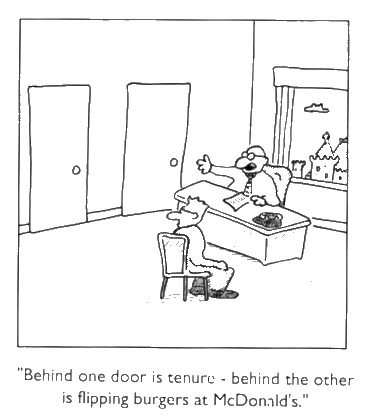
There are two doors in front of you.
You open the left door and get reward \(0\)
\({\color{red}{V(\textit{left}) = 0}\ (\textit{Monte Carlo Estimate})}\)You open the right door and get reward \(+1\)
\({\color{red}{V(\textit{right}) = +1}}\)You open the right door and get reward \(+3\)
\({\color{red}{V(\textit{right}) = +2}}\)You open the right door and get reward \(+2\)
\({\color{red}{V(\textit{right}) = +2}}\)
\(\vdots\)
You may never explore left door again!
- i.e. are you sure you’ve chosen the best door?
\(\varepsilon\)-Greedy Exploration
The simplest idea for ensuring continual exploration:
All \(m\) actions are tried with non-zero probability
with probability \(1 - \varepsilon\) choose the best action, greedily
with probability \(\varepsilon\) choose a random
\[ \pi(a \mid s) = \begin{cases} \dfrac{\varepsilon}{{\color{blue}{m}}} + 1 - \varepsilon & \text{if } a^* = \arg\max\limits_{a \in \mathcal{A}} Q(s,a) \\ \dfrac{\varepsilon}{{\color{blue}{m}}} & \text{otherwise} \end{cases} \]
\(\varepsilon\)-Greedy Policy Improvement
\[\begin{align*} q_\pi(s, \pi'(s)) & = \sum_{a \in \mathcal{A}} \pi'(a \mid s) \, q_\pi(s,a) \\[0pt] & = \tfrac{\varepsilon}{m} \sum_{a \in \mathcal{A}} q_\pi(s,a) + (1 - \varepsilon) \max_{a \in \mathcal{A}} q_\pi(s,a) \\[0pt] & \geq \tfrac{\varepsilon}{m} \sum_{a \in \mathcal{A}} q_\pi(s,a) + (1 - \varepsilon) \sum_{a \in \mathcal{A}} \frac{\pi(a \mid s) - \tfrac{\varepsilon}{m}}{1 - \varepsilon} \, q_\pi(s,a) \\[0pt] & = \sum_{a \in \mathcal{A}} \pi(a \mid s) \, q_\pi(s,a) = v_\pi(s) \end{align*}\]
Proof idea: \({\color{blue}{\max_{a \in \mathcal{A}} q_\pi(a,a)}}\) is at least as good as any weighted sum of all of your actions; therefore from the policy improvement theorem, \(v_{\pi'}(s) \;\geq\; v_\pi(s)\)
Monte-Carlo Policy Iteration

Policy evaluation Monte-Carlo policy evaluation, \(Q=q_\pi\)
Policy improvement \({\color{red}{\varepsilon-}}\)Greedy policy improvement
Monte-Carlo Control

Every episode:
Policy evaluation Monte-Carlo policy evaluation, \({\color{red}{Q \approx q_\pi}}\)
- Not necessary to fully evaluate policy every time, going all the way to the top, instead, immediately improve policy for every episode
Policy improvement \(\varepsilon-\)Greedy policy improvement
Greedy in the Limit with Infinite Exploration (GLIE)
For example, \(\varepsilon\)-greedy is GLIE if \(\varepsilon_k\) reduces to zero at \(\varepsilon_k = \tfrac{1}{k}\)
- i.e. decay \(\varepsilon\) over time according to a hyperbolic schedule
Note that the term \(\mathbf{1}(S_t = s)\) is an indicator function that equals \(1\) if the condition inside is true, and \(0\) otherwise.
\[ \mathbf{1}(S_t = s) = \begin{cases} 1, & \text{if } S_t = s \\ 0, & \text{otherwise} \end{cases} \]
It acts as a selector that ensures the update is applied only to the state currently being visited.
- The boldface notation \(\mathbf{1}(S_t = s)\) simply emphasises that this is a function, not a constant.
GLIE Monte-Carlo Control
Sample \(k\)th episode using \(\pi\): \(\{ S_1, A_1, R_2, \ldots, S_T \} \sim \pi\)
For each state \(S_t\) and action \(A_t\) in the episode update an incremental mean,
\[\begin{align*} N(S_t, A_t) \;\;& \leftarrow\;\; N(S_t, A_t) + 1\\[0pt] Q(S_t, A_t) \;\;& \leftarrow\;\; Q(S_t, A_t) + \frac{1}{N(S_t, A_t)} \Big( G_t - Q(S_t, A_t) \Big) \end{align*}\]
Improve policy based on new action–value function, replacing Q values at each step
\[\begin{align*} \varepsilon \;& \leftarrow\; \tfrac{1}{k}\\[0pt] \pi \;& \leftarrow\; \varepsilon\text{-greedy}(Q) \end{align*}\]
- In practice don’t need to store \(\pi\), just store \(Q\) (\(\pi\) becomes implicit)
Converges to the optimal policy, \(\pi_\ast\)
Every episode Monte-Carlo is substantially more efficient than running multiple episodes at each step
Back to the Blackjack Example

Monte-Carlo Control in Blackjack
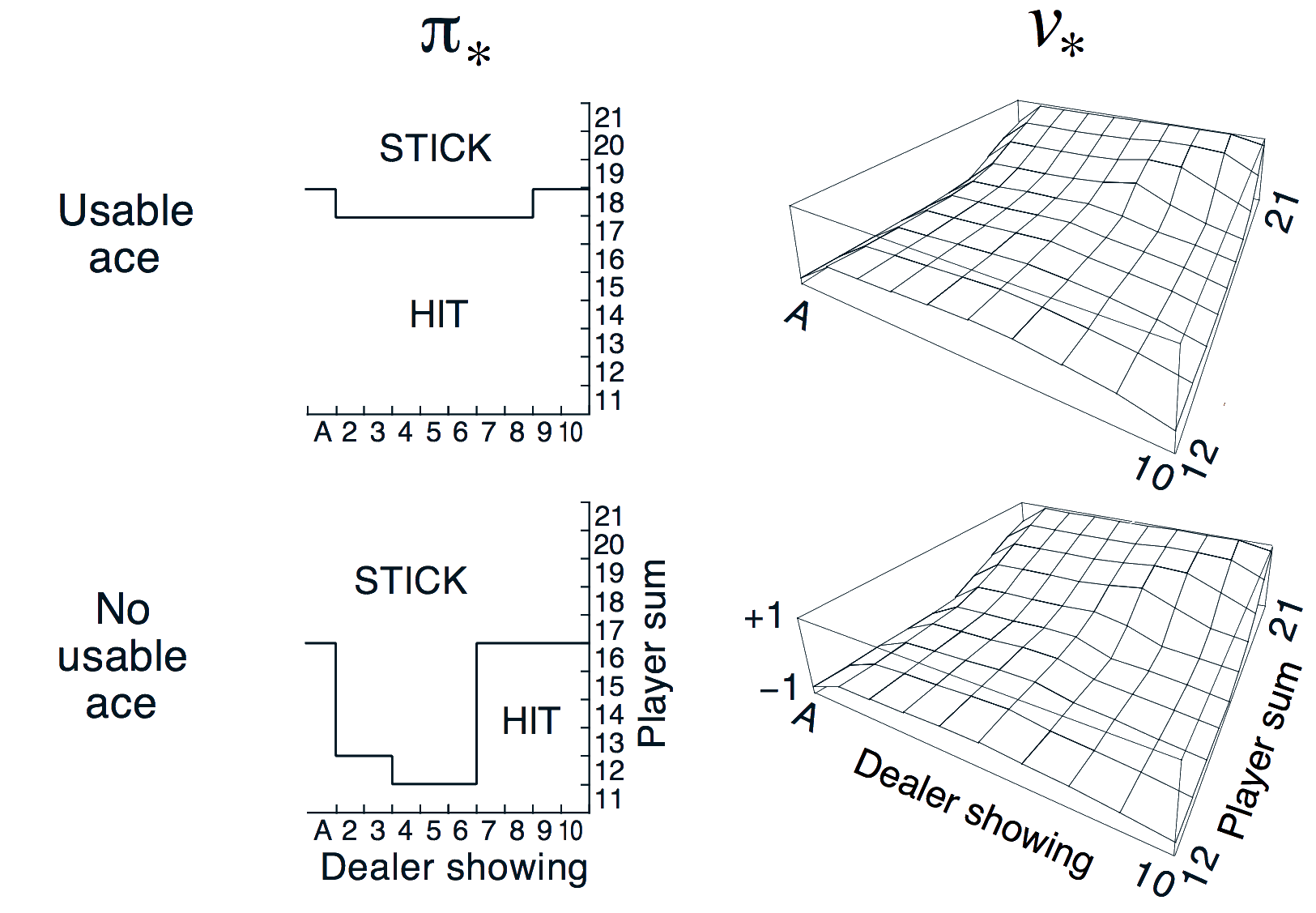
Monte-Carlo Control algorithm finds the optimal policy!
(Note: Stick is equivalent to hold in this Figure)
On-Policy Temporal-Difference Learning
MC versus TD Control (Gain efficiency by Bootstrapping)
Temporal-difference (TD) learning has several advantages over Monte-Carlo (MC)
Lower variance
Online (including non-terminating)
Incomplete sequences
Natural idea: use TD instead of MC in our control loop
Apply TD to \(Q(S,A)\)
Use \(\varepsilon\)-greedy policy improvement
Update every time-step
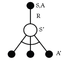
Updating Action-Value Functions with Sarsa

\[ Q(S,A) \;\leftarrow\; Q(S,A) + \alpha \Big({\color{blue}{R + \gamma Q(S',A')}} - Q(S,A) \Big) \]
Starting in state-action pair \(S,A\), sample reward \(R\) from environment, then sample our own policy in \(S^{\prime}\) for \(A^{\prime}\) (note \(S^{\prime}\) is chosen by the environment)
- Moves \(Q(S,A)\) value in direction of TD Target - \(Q(S,A)\) (as in Bellman equation for Q).
On-Policy Control with Sarsa
Every time-step:
Policy evaluation Sarsa, \(Q \approx q_\pi\)
Policy improvement \(\varepsilon-\)Greedy policy improvement
Sarsa Algorithm for On-Policy Control
RHS of \(Q(S,A)\) update is on-policy version of Bellman equation—expectation of what happens in environment to state \(S^{\prime}\) and what happens under our own policy from that state \(S^{\prime}\) onwards.
Convergence of Sarsa (Stochastic optimisation theory)
Tells us that step sizes must be sufficiently large to move us as far as you want; and changes to step sizes must result in step eventually vanishing
Windy Gridworld Example
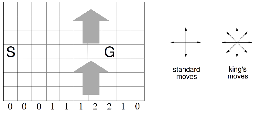
Numbers under each column is how far you get blown up per time step
- Reward \(= -1\) per time-step until reaching goal
(Undiscounted and uses fixed step size \(\alpha\) in this example)
Sarsa on the Windy Gridworld

Episodes completed (vertical axis) versus time steps (horizontal axis)
\(n\)-Step Sarsa (Bias-variance trade-off)
Consider the following \(n\)-step returns for \(n = 1, 2, \infty\):
\[\begin{align*} {\color{red}{n}} & {\color{red}{= 1\ \ \ \ \ \text{(Sarsa)}}} & q_t^{(1)} & = R_{t+1} + \gamma Q(S_{t+1})\\[0pt] {\color{red}{n}} & {\color{red}{= 2}} & q_t^{(2)} & = R_{t+1} + \gamma R_{t+2} + \gamma^2 Q(S_{t+2})\\[0pt] & {\color{red}{\vdots}} & & \vdots \\[0pt] {\color{red}{n}} & {\color{red}{= \infty\ \ \ \ \text{(MC)}}} & q_t^{(\infty)} & = R_{t+1} + \gamma R_{t+2} + \ldots + \gamma^{T-1} R_T \end{align*}\]
Define the \(n\)-step Q-return:
\[ q_t^{(n)} = R_{t+1} + \gamma R_{t+2} + \ldots + \gamma^{n-1} R_{t+n} + \gamma^n Q(S_{t+n}) \]
\(n\)-step Sarsa updates \(Q(s,a)\) towards the \(n\)-step Q-return:
\[ Q(S_t, A_t) \;\leftarrow\; Q(S_t, A_t) + \alpha \Big( q_t^{(n)} - Q(S_t, A_t) \Big) \]
\(n=1\): high bias, low variance
\(n=\infty\): no bias, high variance
Forward View Sarsa(\(\lambda\))

We can do the same thing for control as we did in model-free prediction:
The \(q^\lambda\) return combines all \(n\)-step Q-returns \(q_t^{(n)}\)
Using weight \((1 - \lambda)\lambda^{n-1}\):
\[ q_t^\lambda \;=\; (1 - \lambda) \sum_{n=1}^{\infty} \lambda^{n-1} q_t^{(n)} \]
Forward-view Sarsa(\(\lambda\)):
\[ Q(S_t, A_t) \;\leftarrow\; Q(S_t, A_t) + \alpha \Big( q_t^\lambda - Q(S_t, A_t) \Big) \]
Backward View Sarsa(\(\lambda\))
Just like TD(\(\lambda\)), we use eligibility traces in an online algorithm
- However Sarsa(\(\lambda\)) has one eligibility trace for each state–action pair
\[\begin{align*} E_0(s,a) & = 0 \\[0pt] E_t(s,a) & = \gamma \lambda E_{t-1}(s,a) + \mathbf{1}(S_t = s, A_t = a) \end{align*}\]
\(Q(s,a)\) is updated for every state \(s\) and action \(a\)
- In proportion to TD-error \(\delta_t\) and eligibility trace \(E_t(s,a)\)
\[ \delta_t = R_{t+1} + \gamma Q(S_{t+1}, A_{t+1}) - Q(S_t, A_t) \]
\[ Q(s,a) \;\leftarrow\; Q(s,a) + \alpha \,\delta_t \, E_t(s,a) \]
Sarsa(\(\lambda\)) Algorithm
Algorithm updates all action-state pairs \(Q(s,a)\) at each step of an episode
Sarsa(\(\lambda\)) Gridworld Example
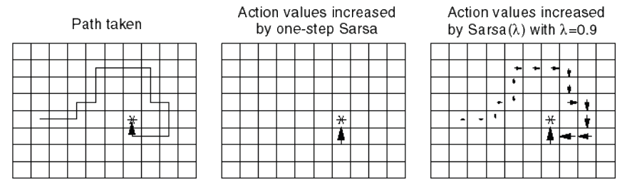
Sarsa(0) Sarsa(\(\lambda\))
Assume initialise action-values to zero
Size of arrow indicates magnitude of \(Q(A,S)\) value for that state
Sarsa updates all action-state pairs \(Q(s,a)\) at each step of episode
Off-Policy Learning
Off-Policy Learning
Evaluate target policy \(\pi(a \mid s)\) to compute \(v_\pi(s)\) or \(q_\pi(s,a)\)
while following a behaviour policy \(\mu(a \mid s)\)
\[ \{ S_1, A_1, R_2, \ldots, S_T \} \sim \mu \]
Why is this important?
Learning from observing humans or other agents (either AI or simulated)
Re-use experience generated from old policies \({\pi_1, \pi_2, \ldots, \pi_{t-1}}\)
Learn about optimal policy while following exploratory policy
Learn about multiple policies while following one policy
Importance Sampling
Estimate the expectation of a different distribution
\[\begin{align*} \mathbb{E}_{X \sim P}[f(X)] \;& =\; \sum P(X) f(X)\\[0pt] & = \sum Q(X) \, \frac{P(X)}{Q(X)} f(X)\\[0pt] & = \mathbb{E}_{X \sim Q} \!\left[ \frac{P(X)}{Q(X)} f(X) \right] \end{align*}\]
A technique for estimating expectations by sampling from different distributions
- Re-weights by dividing and multiplying samples to correct mismatch between expectations of the different distributions
Importance Sampling for Off-Policy Monte-Carlo
Use returns generated from \(\mu\) to evaluate \(\pi\)
Weight return \(G_t\) according to similarity between policies
Multiply importance sampling corrections along entire episode
\[ G_t^{\pi / \mu} = \frac{\pi(A_t \mid S_t)}{\mu(A_t \mid S_t)} \frac{\pi(A_{t+1} \mid S_{t+1})}{\mu(A_{t+1} \mid S_{t+1})} \cdots \frac{\pi(A_T \mid S_T)}{\mu(A_T \mid S_T)} G_t \]
Updates values towards corrected return
\[ V(S_t) \;\leftarrow\; V(S_t) + \alpha \Big( {\color{red}{G_t^{\pi / \mu}}} - V(S_t) \Big) \]
Cannot use if \(\mu\) is zero when \(\pi\) is non-zero
However, importance sampling dramatically increases variance, in case of Monte-Carlo learning
Importance Sampling for Off-Policy TD
Use TD targets generated from \(\mu\) to evaluate \(\pi\)
- Weight TD target \(R + \gamma V(S')\) by importance sampling
Only need a single importance sampling correction
\[ V(S_t) \;\leftarrow\; V(S_t) \;+\; \alpha \Bigg( {\color{red}{ \frac{\pi(A_t \mid S_t)}{\mu(A_t \mid S_t)} \Big( R_{t+1} + \gamma V(S_{t+1}) \Big)}} - V(S_t) \Bigg) \]
Much lower variance than Monte Carlo importance sampling (policies only need to be similar over a single step)
In practice you have to use TD learning when working off-policy (it becomes imperative to bootstrap)
Q-Learning
We now consider off-policy learning of action-values, \(Q(s,a)\)
No importance sampling is required using action-values as you can bootstrap as follows
Next action is chosen using behaviour policy \(A_{t+1} \sim \mu(\cdot \mid S_t)\)
But we consider alternative successor action \(A^{\prime} \sim \pi(\cdot \mid S_t)\)
\(\cdots\) and we update \(Q(S_t, A_t)\) towards value of alternative action
\[ Q(S_t, A_t) \;\leftarrow\; Q(S_t, A_t) + \alpha \Big( {\color{red}{R_{t+1} + \gamma Q(S_{t+1}, A')}} - Q(S_t, A_t) \Big) \]
Q-learning is the technique that works best with off-policy learning
Off-Policy Control with Q-Learning
We can now allow both behaviour and target policies to improve
- The target policy \(\pi\) is greedy w.r.t. \(Q(s,a)\)
\[ \pi(S_{t+1}) = \arg\max_{a'} Q(S_{t+1}, a') \]
- The behaviour policy \(\mu\) is e.g. \(\varepsilon\)-greedy w.r.t. \(Q(s,a)\)
The Q-learning target then simplifies according to:
\[\begin{align*} & R_{t+1} + \gamma Q(S_{t+1}, A')\\[0pt] = & R_{t+1} + \gamma Q\big(S_{t+1}, \arg\max_{a'} Q(S_{t+1}, a')\big)\\[0pt] = & R_{t+1} + \max_{a'} \gamma Q(S_{t+1}, a') \end{align*}\]
Q-Learning Control Algorithm
\[ Q(S,A) \;\leftarrow\; Q(S,A) + \alpha \Big( R + \gamma \max_{a'} Q(S',a') - Q(S,A) \Big) \]
Q-Learning Algorithm for Off-Policy Control
Cliff Walking Example (Sarsa versus Q-Learning)


Relationship between Tree Backup and TD

Relationship between DP and TD
| Dynamic Programming (DP) | Sample Backup (TD) |
|---|---|
| Iterative Policy Evaluation \(V(s) \;\leftarrow\; \mathbb{E}[R + \gamma V(S') \mid s]\) |
TD Learning \(V(S) \;\xleftarrow{\;\alpha\;}\; R + \gamma V(S')\) |
| Q-Policy Iteration \(Q(s,a) \;\leftarrow\; \mathbb{E}[R + \gamma Q(S',A') \mid s,a]\) |
Sarsa \(Q(S,A) \;\xleftarrow{\;\alpha\;}\; R + \gamma Q(S',A')\) |
| Q-Value Iteration \(Q(s,a) \;\leftarrow\; \mathbb{E}\!\left[R + \gamma \max_{a' \in \mathcal{A}} Q(S',a') \;\middle|\; s,a \right]\) |
Q-Learning \(Q(S,A) \;\xleftarrow{\;\alpha\;}\; R + \gamma \max_{a' \in \mathcal{A}} Q(S',a')\) |
where \(x \;\xleftarrow{\;\alpha\;} y \;\;\equiv\;\; x \;\leftarrow\; x + \alpha \,(y - x)\)