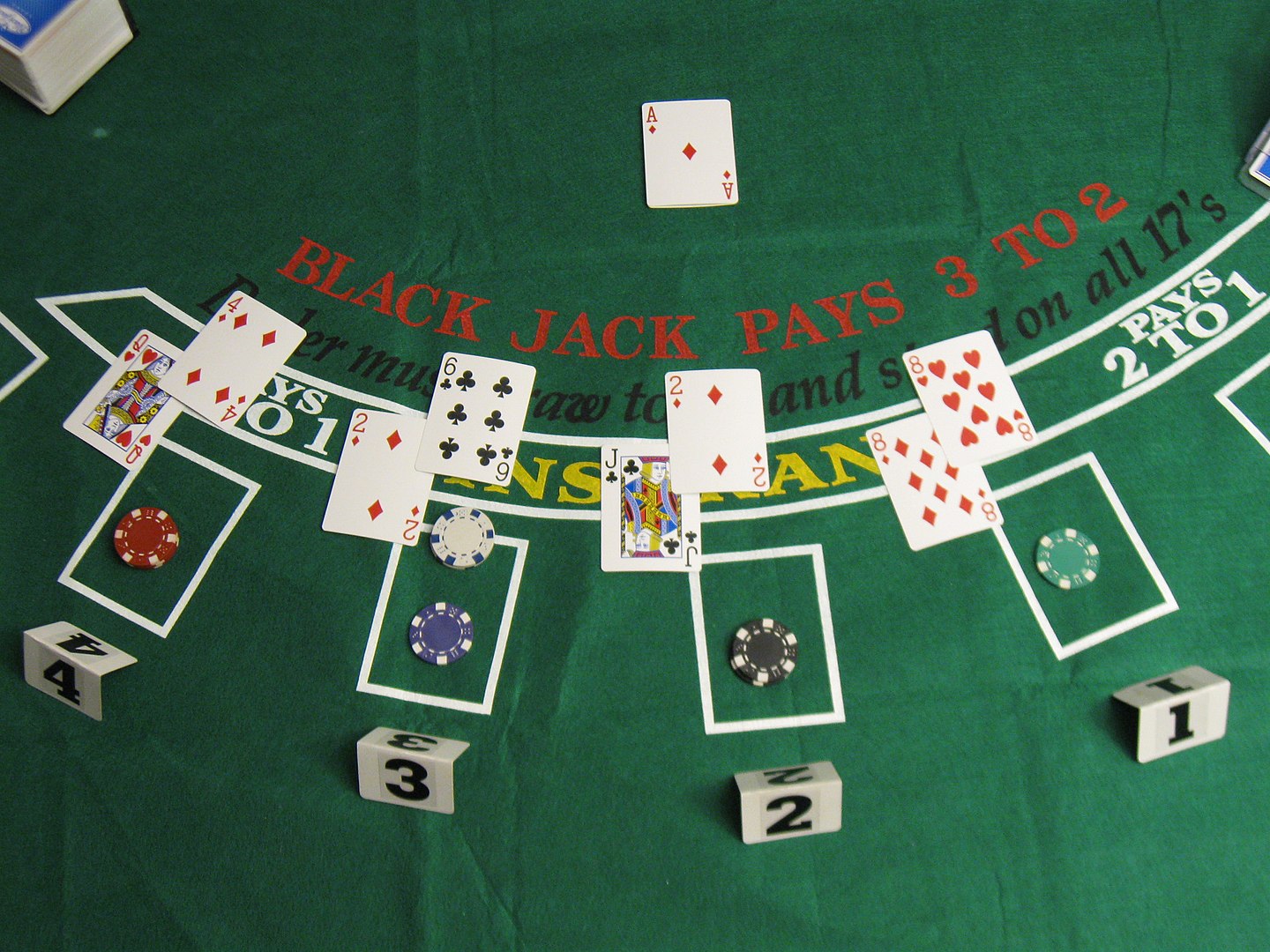
Blackjack Example
States (\(\sim 200\)):
Current sum of cards (\(12-21\))
Dealer’s showing card (Ace\(-10\))
Whether you have a usable ace - (can be counted as \(1\) or \(11\) without busting \(>21\)) (yes/no)
Actions:
Stand: stop receiving cards (and terminate)
Hit: take another card (no replacement)
Transitions:
- You are automatically hit if your sum \(< 12\)
Blackjack Value Function after Monte-Carlo Learning

Policy: stand if sum of cards ≥ 20, otherwise hit
Learning value function directly from experience
Usable ace value is noisier because the state is rarer
Driving Home Example: MC versus TD
Changes recommended by Monte Carlo methods \((\alpha=1)\):
Changes recommended by TD methods \((\alpha=1)\):

Red arrow represent recommended updates by MC and TD respectively
Random Walk Example


Random Walk: MC versus TD

- This demonstrates the benefit of bootstrapping
AB Example
Two states \(A, B\); no discounting; 8 episodes:
\(A, 0, B, 0\)
\(B, 1\)
\(B, 1\)
\(B, 1\)
\(B, 1\)
\(B, 1\)
\(B, 1\)
\(B, 0\)

Clearly, \(V(B)\) = \(\frac{6}{8} = 0.75\), but what about \(V(A)\)?
Monte-Carlo Backup
\[ V(S_t) \;\leftarrow\; V(S_t) + \alpha \big( G_t - V(S_t) \big) \]

Starting at one state, sample one complete trajectory to update the value function
Temporal-Difference Backup
\[ V(S_t) \;\leftarrow\; V(S_t) + \alpha \big( R_{t+1} + \gamma V(S_{t+1}) - V(S_t) \big) \]

In TD backup is just over one step
Tree Search/Dynamic Programming Backup
\[ V(S_t) \;\leftarrow\; \mathbb{E}_\pi \!\left[ R_{t+1} + \gamma V(S_{t+1}) \right] \]

If we know the dynamics of the environment, we can do search and a complete backup over the tree
Unified View of Reinforcement Learning (1)

Unified View of Reinforcement Learning (2)

\(n\)-Step Prediction
Let TD target look \(n\) steps into the future

Large Random Walk Example

- RMS errors vary according to step size \(\alpha\), with the optimum dependent on \(n\)
Averaging \(n\)-Step Returns
We can form mixtures of different \(n\):
e.g. average of \(2\)-step and \(4\)-step returns:
\[ \frac{1}{2} G_t^{(2)} + \frac{1}{2} G_t^{(4)} \]
We can average \(n\)-step returns over different n
- e.g. average the 2-step and 4-step returns
Combines information from two different time-steps
Can we efficiently combine information from all time-steps to be more robust?

\(\lambda\)-return

The \(\lambda\)-return \(G_t^{\lambda}\) combines all \(n\)-step returns \(G_t^{(n)}\)
- Using weight \({\color{red}{(1 - \lambda)\lambda^{\,n-1}}}\)
\[ G_t^{\lambda} \;=\; {\color{red}{(1 - \lambda) \sum_{n=1}^{\infty} \lambda^{\,n-1}}} G_t^{(n)} \]
Forward-view TD(\(\lambda\))
\[ V(S_t) \;\leftarrow\; V(S_t) + \alpha \big( G_t^{\lambda} - V(S_t) \big) \]
TD(\(\lambda\)) Weighting Function

\[ G_t^{\lambda} \;=\; (1 - \lambda) \sum_{n=1}^{\infty} \lambda^{\,n-1} G_t^{(n)} \]
- \(\lambda\)-return is a geometrically weighted return for every \(n\)-step return
Forward View of TD(λ)

Update value function towards the \(\lambda\)-return
Forward-view looks into the future to compute \(G^{\lambda}_t\)
Like MC, can only be computed from complete episodes
We will see shortly how an iterative algorithm achieves the forward view without having to wait until the future
Forward View of TD(λ) on Large Random Walk

We can see using TD(\(\lambda\)), and choosing \(\lambda\) value (left hand side), is more robust than choosing a unique \(n\)-step value (right hand side)
- \(\lambda=1\) is MC and \(\lambda=0\) is TD(\(0\))
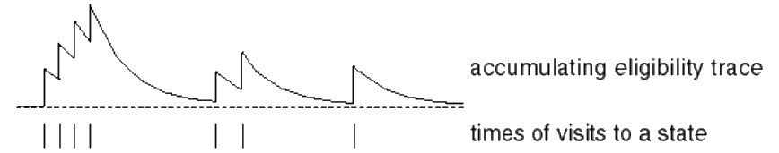
Eligibility Traces

Credit assignment problem: did bell or light cause shock?
Frequency heuristic: assign credit to most frequent states
Regency heuristic: assign credit to most recent states
Eligibility traces combine both heuristics
\[\begin{align*} E_0(s) & = 0\\[2pt] E_t(s) & = \gamma \lambda E_{t-1}(s) + 1(S_t = s) \end{align*}\]

Results of TD search in Go

Generalised Policy Iteration

Alternation converges on optimal policy \(\pi_\ast\)
Policy evaluation Estimate \(v_{\pi}\)
e.g. Iterative policy evaluation, going upPolicy improvement Generate \(\pi^{\prime} \geq \pi\) e.g. Greedy policy improvement, act greedily with respect to value function, going down

Generalised Policy Iteration with Monte-Carlo Evaluation
Policy evaluation 1. Can we use Monte-Carlo policy evaluation to estimate \({\color{blue}{V = v_{\pi}}}\)(running multiple episodes/rollouts)?
Policy improvement 2. Can we do greedy policy improvement with MC evaluation?
Generalised Policy Iteration with Action-Value Function

Policy evaluation We run Monte-Carlo policy evaluation using \({\color{red}{Q=q_\pi}}\)
For each state-action pair \(Q(A,S)\) we take mean return
We do this for all states and actions, i.e. we don’t need model
Policy improvement Greedy policy improvement?
Example of Greedy Action Selection (Bandit problem)

There are two doors in front of you.
You open the left door and get reward \(0\)
\({\color{red}{V(\textit{left}) = 0}\ (\textit{Monte Carlo Estimate})}\)You open the right door and get reward \(+1\)
\({\color{red}{V(\textit{right}) = +1}}\)You open the right door and get reward \(+3\)
\({\color{red}{V(\textit{right}) = +2}}\)You open the right door and get reward \(+2\)
\({\color{red}{V(\textit{right}) = +2}}\)
\(\vdots\)
You may never explore left door again!
- i.e. are you sure you’ve chosen the best door?
Monte-Carlo Policy Iteration

Policy evaluation Monte-Carlo policy evaluation, \(Q=q_\pi\)
Policy improvement \({\color{red}{\varepsilon-}}\)Greedy policy improvement
Monte-Carlo Control

Every episode:
Policy evaluation Monte-Carlo policy evaluation, \({\color{red}{Q \approx q_\pi}}\)
- Not necessary to fully evaluate policy every time, going all the way to the top, instead, immediately improve policy for every episode
Policy improvement \(\varepsilon-\)Greedy policy improvement
Back to the Blackjack Example

Monte-Carlo Control in Blackjack
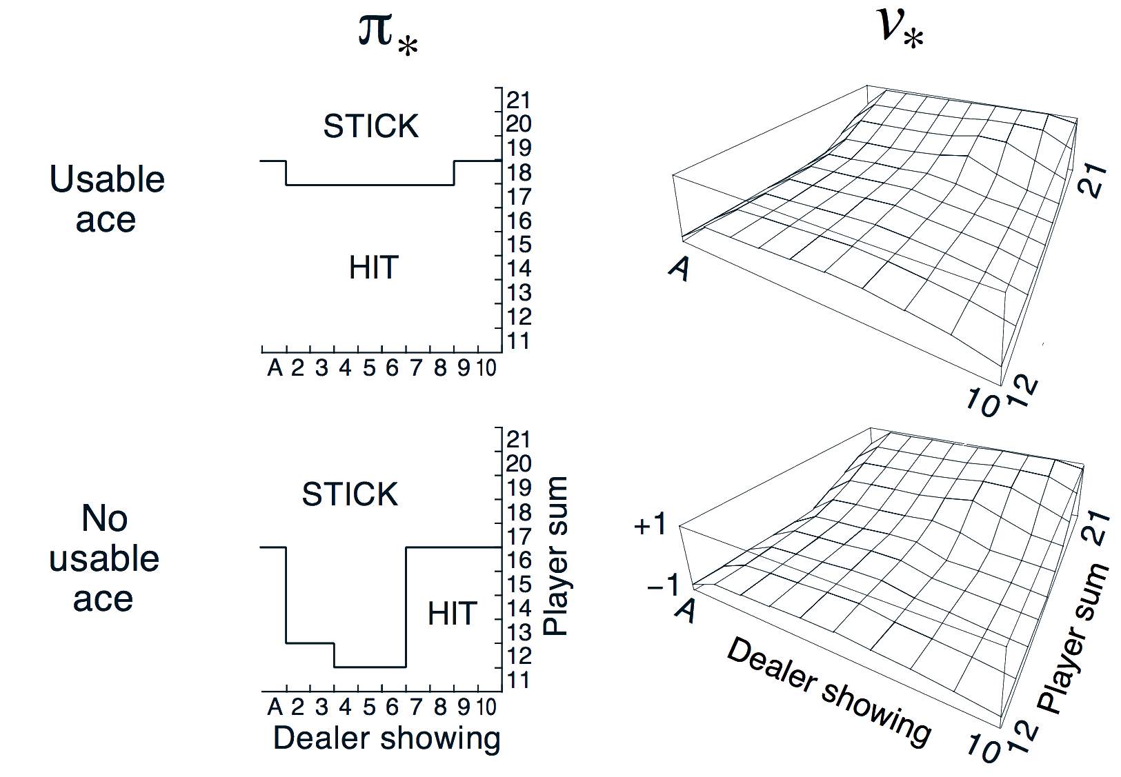
Monte-Carlo Control algorithm finds the optimal policy!
(Note: Stick is equivalent to hold in this Figure)
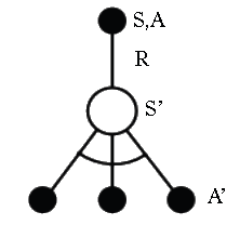
Updating Action-Value Functions with Sarsa

\[ Q(S,A) \;\leftarrow\; Q(S,A) + \alpha \Big({\color{blue}{R + \gamma Q(S',A')}} - Q(S,A) \Big) \]
Starting in state-action pair \(S,A\), sample reward \(R\) from environment, then sample our own policy in \(S^{\prime}\) for \(A^{\prime}\) (note \(S^{\prime}\) is chosen by the environment)
- Moves \(Q(S,A)\) value in direction of TD Target - \(Q(S,A)\) (as in Bellman equation for Q).
On-Policy Control with Sarsa
Every time-step:
Policy evaluation Sarsa, \(Q \approx q_\pi\)
Policy improvement \(\varepsilon-\)Greedy policy improvement
Windy Gridworld Example
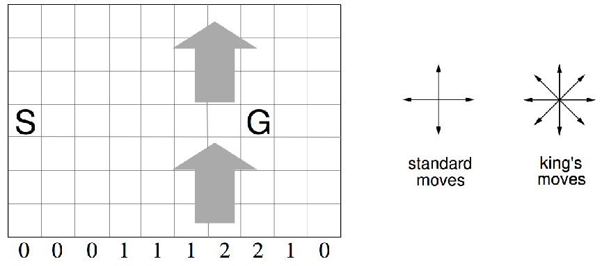
Numbers under each column is how far you get blown up per time step
- Reward \(= -1\) per time-step until reaching goal
(Undiscounted and uses fixed step size \(\alpha\) in this example)
Sarsa on the Windy Gridworld

Episodes completed (vertical axis) versus time steps (horizontal axis)
Forward View Sarsa(\(\lambda\))

We can do the same thing for control as we did in model-free prediction:
The \(q^\lambda\) return combines all \(n\)-step Q-returns \(q_t^{(n)}\)
Using weight \((1 - \lambda)\lambda^{n-1}\):
\[ q_t^\lambda \;=\; (1 - \lambda) \sum_{n=1}^{\infty} \lambda^{n-1} q_t^{(n)} \]
Forward-view Sarsa(\(\lambda\)):
\[ Q(S_t, A_t) \;\leftarrow\; Q(S_t, A_t) + \alpha \Big( q_t^\lambda - Q(S_t, A_t) \Big) \]
Sarsa(\(\lambda\)) Gridworld Example
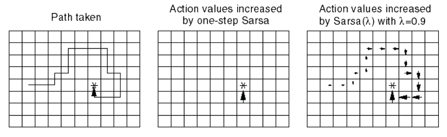
Sarsa(0) Sarsa(\(\lambda\))
Assume initialise action-values to zero
Size of arrow indicates magnitude of \(Q(A,S)\) value for that state
Sarsa updates all action-state pairs \(Q(s,a)\) at each step of episode
Q-Learning Control Algorithm
\[ Q(S,A) \;\leftarrow\; Q(S,A) + \alpha \Big( R + \gamma \max_{a'} Q(S',a') - Q(S,A) \Big) \]
Cliff Walking Example (Sarsa versus Q-Learning)


Relationship between Tree Backup and TD
