8 Integrating Learning and Planning (MCTS)
Slides
This module is also available in the following versions
Model-Based Reinforcement Learning
Last Module: MDPs
This Module: learn model directly from experience
- \(\ldots\) and use planning to construct a value function or policy
Integrates learning and planning into a single architecture
Model-Based Reinforcement Learning
Model-Based and Model-Free RL
Model-Free RL
No model
Learn value function (and/or policy) from experience
Model-Based RL
Learn a model from experience
Plan value function (and/or policy) from model
Lookahead by planning (or thinking) about what the value function will be
Model-Free RL
Model-Based RL
Replace real world with the agent’s (simulated) model of the environment
- Supports rollouts (lookaheads) under imagined actions to reason about what value function will be, without further environment interaction
Model-Based RL (2)

Advantages of Model-Based RL
Advantages:
Can efficiently learn model by supervised learning methods
Can reason about model uncertainty, and even take actions to reduce uncertainty
Disadvantages:
- First learn a model, then construct a value function
\(\;\;\;\Rightarrow\) two sources of approximation error
Learning a Model
What is a Model?
A model \(\mathcal{M}\) is a representation of an MDP \(\langle \mathcal{S}, \mathcal{A}, \mathcal{P}, \mathcal{R} \rangle\), parameterised by \(\eta\)
- We will assume state space \(\mathcal{S}\) and action space \(\mathcal{A}\) are known
So a model \(\mathcal{M} = \langle \mathcal{P}_\eta, \mathcal{R}_\eta \rangle\) represents state transitions
\(\mathcal{P}_\eta \approx \mathcal{P}\) and rewards \(\mathcal{R}_\eta \approx \mathcal{R}\)
\[ S_{t+1} \sim \mathcal{P}_\eta(S_{t+1} \mid S_t, A_t) \]
\[ R_{t+1} = \mathcal{R}_\eta(R_{t+1} \mid S_t, A_t) \]
Typically assume conditional independence between state transitions and rewards
\[ \mathbb{P}[S_{t+1}, R_{t+1} \mid S_t, A_t] \;=\; \mathbb{P}[S_{t+1} \mid S_t, A_t] \; \mathbb{P}[R_{t+1} \mid S_t, A_t] \]
Note you can learn from each (one-step) transition, treating the following step as the supervisor for the prior step.
Model Learning
Goal: estimate model \(\mathcal{M}_\eta\) from experience \(\{S_1, A_1, R_2, \ldots, S_T\}\)
This is a supervised learning problem
\[ \begin{aligned} S_1, A_1 &\;\to\; R_2, S_2 \\ S_2, A_2 &\;\to\; R_3, S_3 \\ &\;\vdots \\ S_{T-1}, A_{T-1} &\;\to\; R_T, S_T \end{aligned} \]
Learning \(s,a \to r\) is a regression problem
Learning \(s,a \to s'\) is a density estimation problem
Pick loss function, e.g. mean-squared error, KL divergence, …
Find parameters \(\eta\) that minimise empirical loss
Examples of Models
Table Lookup Model
Linear Expectation Model
Linear Gaussian Model
Gaussian Process Model
Deep Belief Network Model
\(\cdots\) almost any supervised learning model
Table Lookup Model
Model is an explicit MDP, \(\hat{\mathcal{P}}, \hat{\mathcal{R}}\)
- Count visits \(N(s,a)\) to each state–action pair (parametric approach)
\[ \begin{align*} \hat{\mathcal{P}}^{a}_{s,s'} & = \frac{1}{N(s,a)} \sum_{t=1}^T \mathbf{1}(S_t, A_t, S_{t+1} = s, a, s')\\[0pt] \hat{\mathcal{R}}^{a}_{s} & = \frac{1}{N(s,a)} \sum_{t=1}^T \mathbf{1}(S_t, A_t = s, a)\, R_t \end{align*} \]
- Alternatively (a simple non-parametric approach)
- At each time-step \(t\), record experience tuple \(\langle S_t, A_t, R_{t+1}, S_{t+1} \rangle\)
- To sample model, randomly pick tuple matching \(\langle s,a,\cdot,\cdot \rangle\)
AB Example (Revisited) - Building a Model
Two states \(A,B\); no discounting; \(8\) episodes of experience
\(A, 0, B, 0\)
\(B, 1\)
\(B, 1\)
\(B, 1\)
\(B, 1\)
\(B, 1\)
\(B, 1\)
\(B, 0\)

We have constructed a table lookup model from the experience
Planning with a Model
Planning with a Model
Given a model \(\mathcal{M}_\eta = \langle \mathcal{P}_\eta, \mathcal{R}_\eta \rangle\)
- Solve the MDP \(\langle \mathcal{S}, \mathcal{A}, \mathcal{P}_\eta, \mathcal{R}_\eta \rangle\)
Using favourite planning algorithm
Value iteration
Policy iteration
Tree search
\(\cdots\)
Sample-Based Planning
A simple but powerful approach to planning is to use the model only to generate samples
Sample experience from model
\[ \begin{align*} S_{t+1} & \sim \mathcal{P}_\eta(S_{t+1} \mid S_t, A_t)\\[0pt] R_{t+1} & = \mathcal{R}_\eta(R_{t+1} \mid S_t, A_t) \end{align*} \]
Apply model-free RL to samples, e.g.:
Q-learning
Monte-Carlo control or Sarsa
Sample-based planning methods are often more efficient
Back to the AB Example
Construct a table-lookup model from real experience
Apply model-free RL to sampled experience
Real experience
\(A, 0, B, 0\)
\(B, 1\)
\(B, 1\)
\(B, 1\)
\(B, 1\)
\(B, 1\)
\(B, 1\)
\(B, 0\)
Sampled experience
\(B, 1\)
\(B, 0\)
\(B, 1\)
\(A, 0, B, 1\)
\(B, 1\)
\(A, 0, B, 1\)
\(B, 1\)
\(B, 0\)
e.g. Monte-Carlo learning: \(V(A) = 1\); \(V(B) = 0.75\)
We can sample as many trajectories as we want from the model, unlike from the environment
- we essentially have infinite data
Planning with an Inaccurate Model
Given an imperfect model \(\langle \mathcal{P}_\eta, \mathcal{R}_\eta \rangle \ne \langle \mathcal{P}, \mathcal{R} \rangle\)
Performance of model-based RL is limited to optimal policy
for approximate MDP \(\langle \mathcal{S}, \mathcal{A}, \mathcal{P}_\eta, \mathcal{R}_\eta \rangle\)i.e. Model-based RL is only as good as the estimated model
When the model is inaccurate, planning process will compute a sub-optimal policy
Solution 1: when model is wrong, use model-free RL
Solution 2: reason explicitly about model uncertainty (e.g. Bayesian approach)
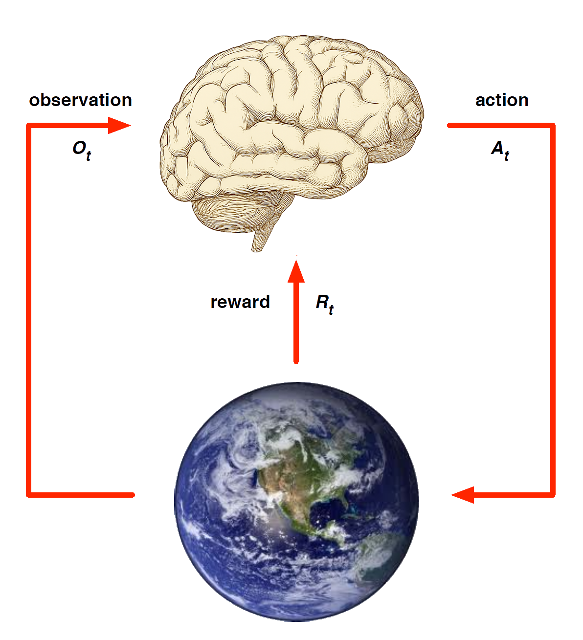
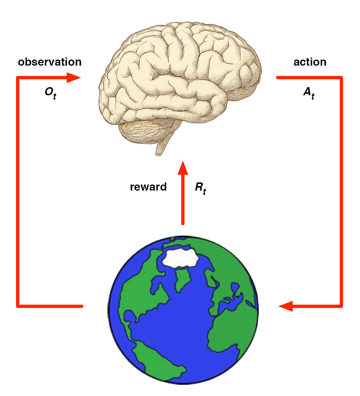
Real and Simulated Experience
We consider two sources of experience
Real experience Sampled from environment (true MDP)
\[ \begin{align*} S' & \sim \mathcal{P}^a_{s,s'}\\[0pt] R & = \mathcal{R}^a_{s} \end{align*} \]
Simulated experience Sampled from model (approximate MDP)
\[ \begin{align*} S' & \sim \mathcal{P}_\eta(S' \mid S, A) \\[0pt] R & = \mathcal{R}_\eta(R \mid S, A) \end{align*} \]
Integrating Learning and Planning
Model-Free RL
No model
Learn value function (and/or policy) from real experience
Model-Based RL (using Sample-Based Planning)
Learn a model from real experience
Plan value function (and/or policy) from simulated experience
Integrated Architectures
Learn a model from real experience
Learn and plan value function (and/or policy) from real and simulated experience
Simulation-Based Search
Simulation-Based Search (1)
Forward search algorithms select the best action by look-ahead
They build a search tree with the current state \(s_t\) at the root
Using a model of the MDP to look ahead

No need to solve whole MDP, just sub-MDP starting from now
Simulation-Based Search (2)
Forward search paradigm using sample-based planning
Simulate episodes of experience from now with the model
Apply model-free RL to simulated episodes

Simulation-Based Search (3)
Simulate episodes of experience from now with the model
\[ \{ s_t^k, A_t^k, R_{t+1}^k, \ldots, S_T^k \}_{k=1}^K \;\sim\; \mathcal{M}_\nu \]
Apply model-free RL to simulated episodes
Monte-Carlo control \(\;\to\;\) Monte-Carlo search
Sarsa \(\;\to\;\) TD search
Simple Monte-Carlo Search
Given a model \(\mathcal{M}_\nu\), and a simulation policy \(\pi\)
- For each action \(a \in \mathcal{A}\)
- Simulate \(K\) episodes from current (real) state \(s_t\)
\[ \{ s_t, a, R_{t+1}^k, S_{t+1}^k, A_{t+1}^k, \ldots, S_T^k \}_{k=1}^K \;\sim\; \mathcal{M}_\nu, \pi \]
- Evaluate actions by mean return (Monte-Carlo evaluation)
\[ Q(\textcolor{blue}{s_t, a}) = \frac{1}{K} \sum_{k=1}^K G_t \;\overset{P}{\to}\; q_\pi(s_t, a) \]
- Select current (real) action with maximum value \(a_t = \arg\max_{a \in \mathcal{A}} Q(s_t, a)\)
Monte-Carlo Tree Search (Evaluation)
Given a model \(\mathcal{M}_\nu\), simulate \(K\) episodes from current state \(s_t\) using current simulation policy \(\pi\)
\[ \{ {\color{red}{s_t}}, A_t^k, R_{t+1}^k, S_{t+1}^k, \ldots, S_T^k \}_{k=1}^K \;\sim\; \mathcal{M}_\nu, \pi \]
Build a search tree containing visited states and actions
Evaluate states \(Q(s,a)\) by mean return of episodes from each pair \(s,a\)
\[ Q(\textcolor{red}{s,a}) = \frac{1}{N(s,a)} \sum_{k=1}^K \sum_{u=t}^T \mathbf{1}(S_u, A_u = s,a) \, G_u \;\;\overset{P}{\to}\;\; q_\pi(s,a) \]
After search is finished, select current (real) action with maximum value in search tree \(a_t = \arg\max_{a \in \mathcal{A}} Q(s_t, a)\)
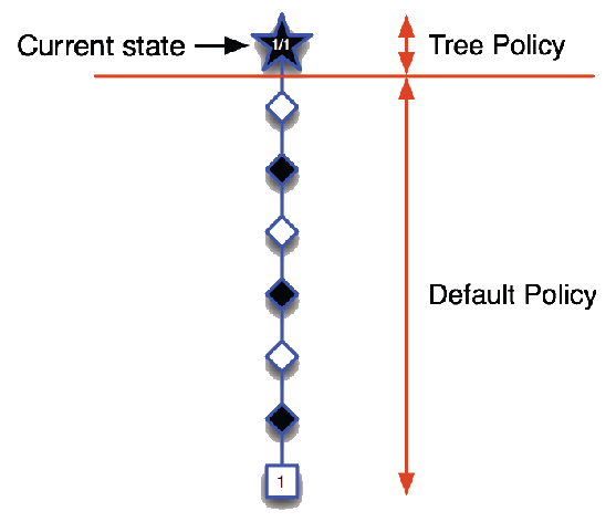
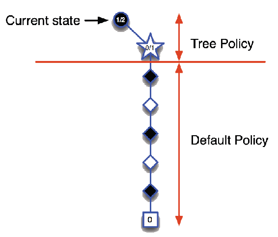
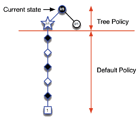
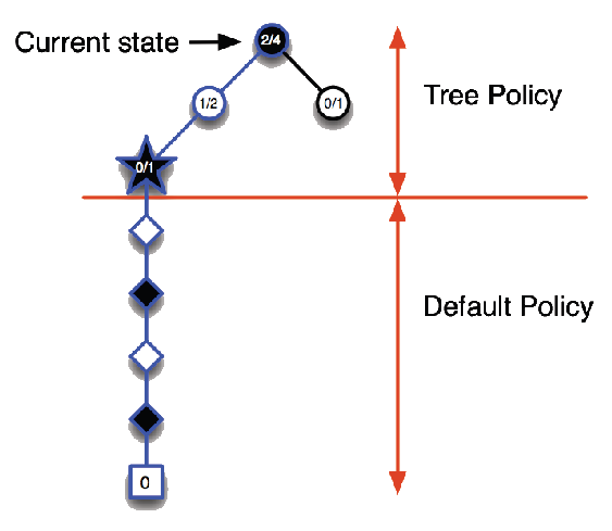
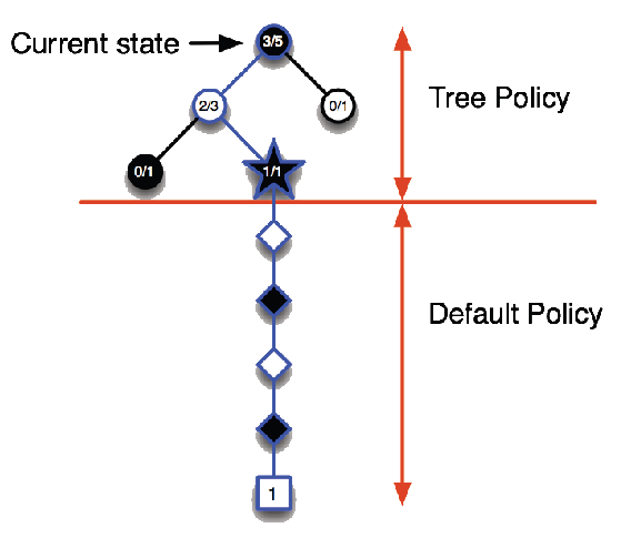
Monte-Carlo Tree Search (Simulation)
In MCTS, the simulation policy \(\pi\) improves
Each simulation consists of two phases (in-tree, out-of-tree)
Tree policy (improves): pick actions to maximise \(Q(S,A)\)
Default policy (fixed): pick actions randomly
Monte-Carlo control applied to simulated experience
- Converges on the optimal search tree,
\(Q(S,A) \;\to\; q_*(S,A)\)
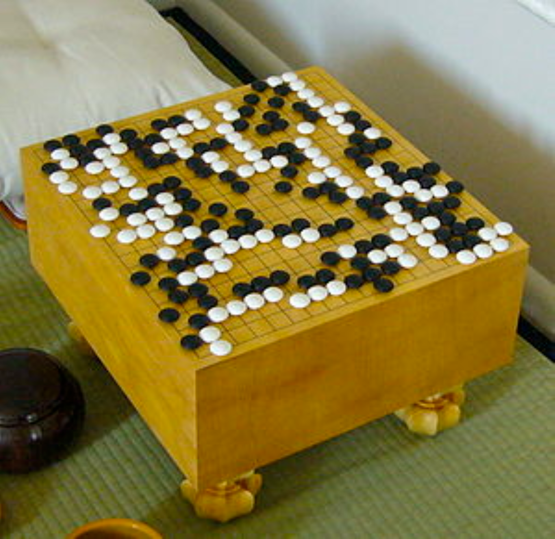
Example: The Game of Go
Example: The Game of Go
The ancient oriental game of Go is \(2,500\) years old
Considered to be the hardest classic board game
Considered a grand challenge task for AI (John McCarthy)
Traditional game-tree search has failed in Go
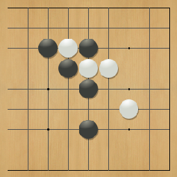
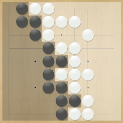
Rules of Go
Usually played on 19x19, also 13x13 or 9x9 board
Simple rules, complex strategy
Black and white place down stones alternately
Surrounded stones are captured and removed
The player with more territory wins the game
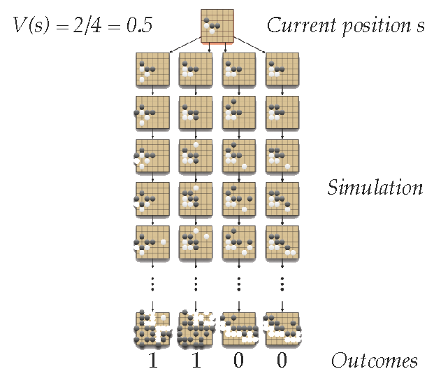
Position Evaluation in Go
How good is a position \(s\)?
- Reward function (undiscounted):
\[ \begin{align*} R_t & = 0 \quad \text{for all non-terminal steps } t < T\\[0pt] R_T & = \begin{cases} 1 & \text{if Black wins} \\ 0 & \text{if White wins} \end{cases} \end{align*} \]
Policy \(\pi = \langle \pi_B, \pi_W \rangle\) selects moves for both players
Value function (how good is position \(s\)):
\[ \begin{align*} v_\pi(s) & = \mathbb{E}_\pi \left[ R_T \mid S = s \right] = \mathbb{P}[ \text{Black wins} \mid S = s ]\\[0pt] v_*(s) & = \max_{\pi_B} \min_{\pi_W} v_\pi(s) \end{align*} \]
Monte-Carlo Evaluation in Go
Applying Monte-Carlo Tree Search (1)
Applying Monte-Carlo Tree Search (2)
Applying Monte-Carlo Tree Search (3)
Applying Monte-Carlo Tree Search (4)
Applying Monte-Carlo Tree Search (5)
Advantages of MC Tree Search
Highly selective best-first search
Evaluates states dynamically (unlike e.g. dynamic programming which does not use trees)
Uses sampling to break curse of dimensionality
Works for “black-box” models (only requires samples)
- Computationally efficient, anytime, parallelisable