05 Markov Decision Processes (MDPs)

Slides

This module is also available in the following versions

Intro to Reinforcement Learning (RL)

What is RL?

A machine learning paradigm in which agents learn to make sequential decisions in an uncertain environment, guided by rewards and penalties.

Agents = perspectives: limited knowledge, outcomes influence environment
Uncertainty comes from environment (single agent RL) or other agents (multi-agent RL)
Learning and reward-seeking are bundled: agents learn by reinforcing rewarding behaviors
Solutions balance exploration of options and exploitation of current best knowledge

Learning and Planning

Two fundamental problems in sequential decision making

Planning (first half of COMP90054):

A model of the environment is known
The agent performs computations with its model (without any external interaction)
The agent improves its policy through search, deliberation, reasoning, and introspection

Reinforcement Learning (this half of COMP90054):

The environment is initially unknown
The agent interacts with the environment
The agent improves its policy

Atari Example

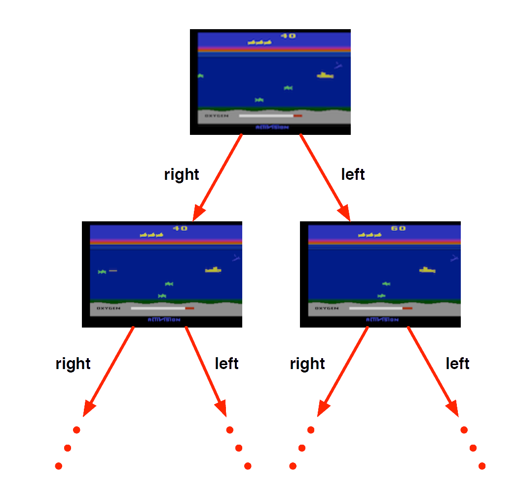
Atari Example: Planning

Rules of the game are known

Can query emulator (simulator)

perfect model inside agent’s brain

If I take action $a$ from state $s$:

what would the next state $s'$ be?
what would the score be?

Plan ahead to find optimal policy, e.g. heuristic tree search, novelty etc.

Atari Example (without emulator): Reinforcement Learning

Rules of the game are unknown
Pick joystick actions, only see pixels & scores
Learn directly from interactive game-play

Examples of Reinforcement Learning

Making a humanoid robot walk
Fine tuning LLMs using human/AI feedback
Optimising operating system routines
Controlling a power station
Managing an investment portfolio

See appendix for more details

Key Concepts in RL

Decision-making under uncertainty (decision theory)
Maximising expected rewards
Balancing exploration and exploitation

Decision-making under uncertainty

	☀️ Sunny	🌧️ Raining
Bring ☂️	😒	🙂
Don’t bring ☂️	😀	😭

Exp(☂️) = P(☀️)·U(😒) + P(🌧️)·U(🙂)

Reward Hypothesis

Goals are characterised as the maximisation of expected cumulative reward.

Example of Rewards

Make a humanoid robot walk
- -x reward for falling
- +y reward for forward motion
Control inventory in a warehouse
- -x reward for stock-out penalty (lost sales)
- -y reward for holding costs (inventory)
- +z reward for sales revenue

Sequential Decision Making

Goal: select actions to maximise total future reward

Actions may have long term consequences
Reward may be delayed
It may be better to sacrifice immediate reward to gain more long-term reward

Examples:

A financial investment (may take months to mature)
A game-playing agent for a game scored at the end of many rounds of play

Exploration and Exploitation

Reinforcement learning is like trial-and-error learning

The agent should discover a good policy…

…from its experiences of the environment…

…without losing too much reward along the way.

Exploration finds more information about the environment
Exploitation exploits known information to maximise reward

Examples

Restaurant Selection
Exploitation Go to your favourite restaurant
Exploration Try a new restaurant
Online Banner Advertisements
Exploitation Show the most successful advert
Exploration Show a different advert
Gold exploration
Exploitation Drill core samples at the best known location
Exploration Drill at a new location

Markov Decision Processes (MDPs)

New Modelling Paradigm

CLASSICAL PLANNING

Set of states $S$

Initial state $s_0$

Actions $A(s)$

Transition function $s' = f(a, s)$

Goals $S_G \subseteq S$

Action costs $c(a, s)$

MDPs

Set of states $S$

Initial state $s_0$

Actions $A(s)$

Transition probabilities $P_a(s' \mid s)$

Reward function $r(s, a, s')$ positive or negative of transitioning from state $s$ to state $s'$

Discount factor $0 \leq \gamma \leq 1$

Markov Decision Process (MDP)

Definition

A Markov Decision Process is a tuple $<\mathcal{S}, \mathcal{A}, \mathcal{P}, \mathcal{R}, \gamma>$

$\mathcal{S}$ is a finite set of states
$\mathcal{{A}}$ is a finite set of actions
$\mathcal{P}$ is a state transition probability matrix, $P^{a}_{s,s'} = \mathbb{P} [S_{t+1} = s' | S_t = s, A_t = a]$
$\mathcal{R}$ is a reward function, $\mathcal{R}^{a}_{s, s'} = \mathbb{E}[R_{t+1} | S_t = s, A_t = {a}, S_{t+1} = s' ]$
$\gamma$ is a discount factor $\gamma \in [0,1]$.

Example: Gridworld

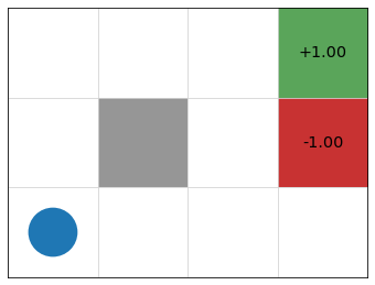
states = cells
actions = up, down, left, right, 10% chance of 90$\degree$ error
reward $r(s) = 0$ for non-terminal nodes
discount factor $\gamma = 0.9$

Episodes

An episode, history, or trajectory through an MDP is the sequence of states and actions that occur as an agent traverses an MDP.

Example:

state = (1, 1), (try to) go up,

state = (2, 1), go right,

state = (3, 1), go up,

state = (3, 2), (try to) go up

state = (4, 2) TERMINAL

Return

Definition: Return

The return $G_t$ is the total discounted reward from time-step $t$. \[ G_t \;=\; R_{t+1} \;+\; \gamma R_{t+2} \;+\; \dots \;=\; \sum_{k=0}^{\infty} \gamma^k R_{t+k+1} \]

The discount $\gamma \in [0, 1]$ is the present value of future rewards
The value of receiving reward $R$ after $k+1$ time-steps is $\gamma^k R$.
This values immediate reward above delayed reward
- $\gamma$ close to $0$ leads to “myopic” evaluation
- $\gamma$ close to $1$ leads to “far-sighted” evaluation

Why discount?

Why are Markov reward/decision processes often discounted?

Avoids infinite returns for infinite (or arbitrarily long) trajectories
Reflects uncertainty about the future when anticipating outcomes
Expresses if and how we value efficiency/speed when ranking solutions

Modelling Considerations for MDPs

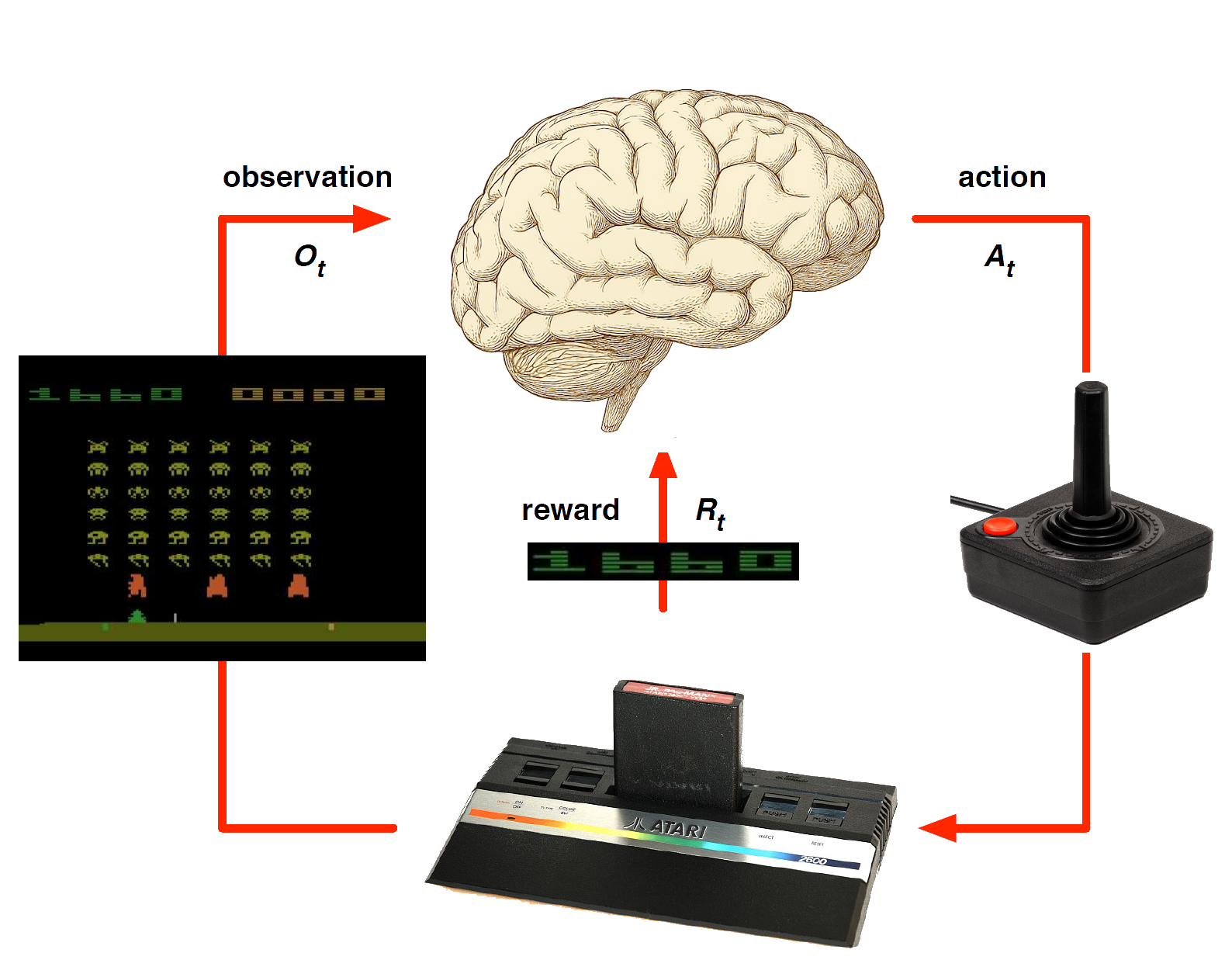
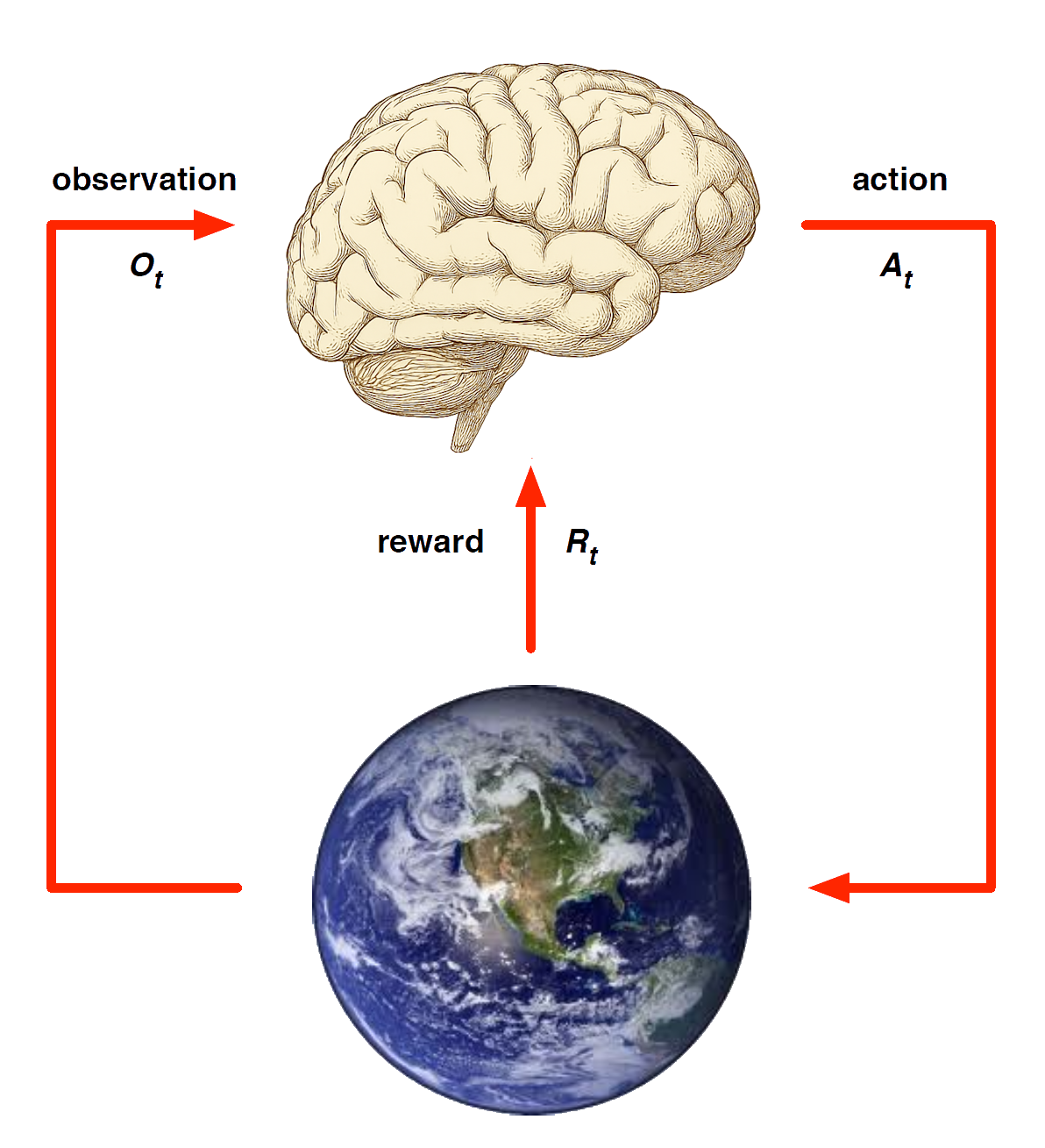
Agent and Environment

At each step $t$ the agent:

Executes action $A_t$
Receives observation $O_t$
Receives scalar reward $R_t$

The environment:

Receives action $A_t$

Emits observation $O_{t+1}$
Emits scalar reward $R_{t+1}$
$t$ increments at env. step

History and State

The history is sequence of observations, actions, rewards

\[ H_t = O_1,R_1,A_1, \ldots A_{t-1}, O_t, R_t \] - i.e. the stream of a robot’s actions, observations and rewards up to time $t$

What happens next depends on the history:

The agent selects actions, and
the environment selects observations/rewards.

State is the information used to determine what happens next.

Formally, a state is a function of the history: $S_t = f(H_t )$

Environment State

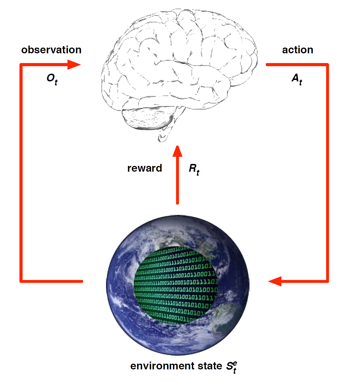
The environment state $S^e_t$ is the environment’s private representation

i.e. data environment uses to pick the next observation/reward

The environment state is not usually visible to the agent

Even if $S^e_t$ is visible, it may contain irrelevant info

Agent State

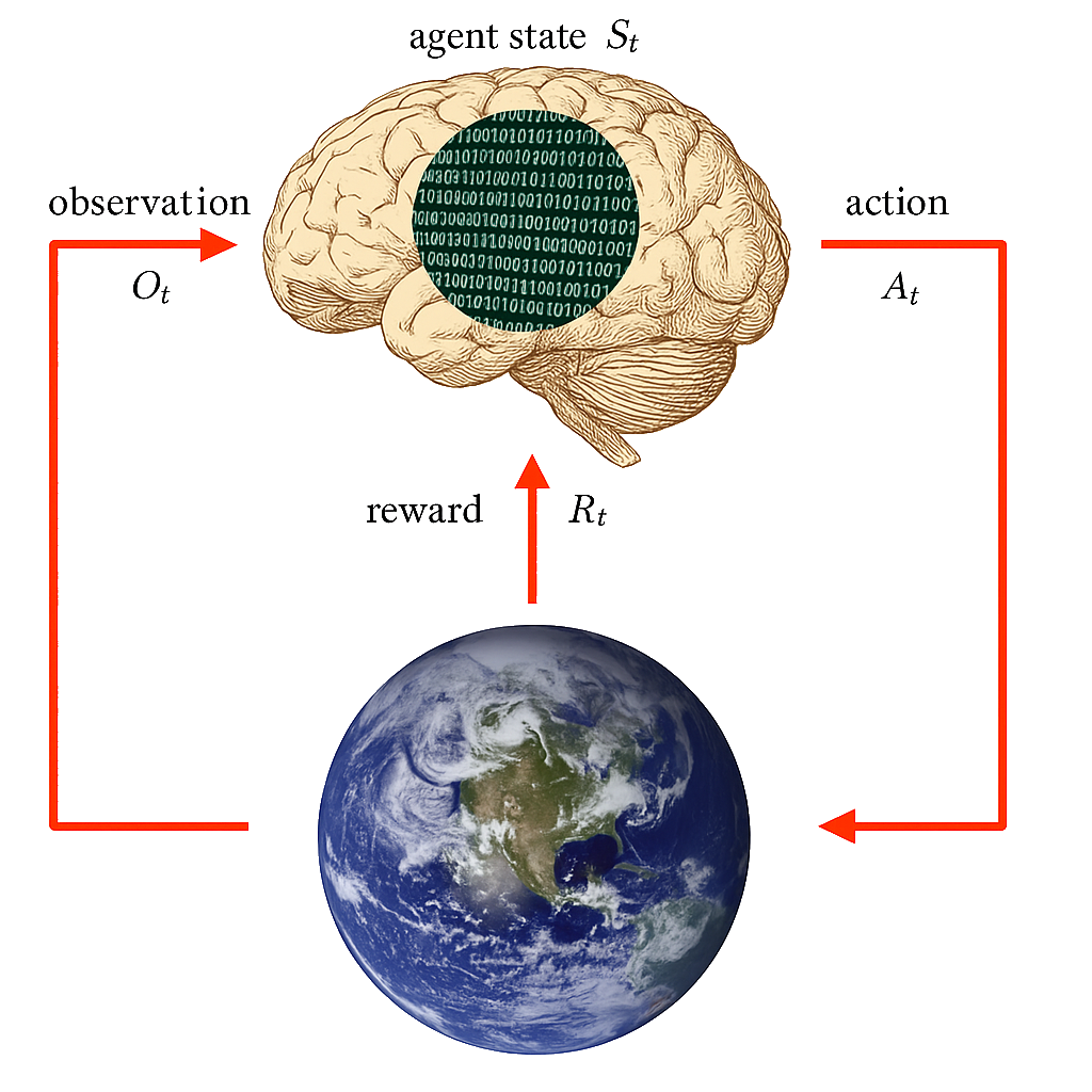
The agent state $S^a_t$ is the agent’s internal representation

i.e. information the agent uses to pick the next action
i.e. information used by reinforcement learning algorithms

It can be any function of history: $S^a_t = f(H_t)$

Markov State

A Markov state (a.k.a. Information state) contains all useful information from the history.

Definition: A state $S_t$ is Markov if and only if \[ \mathbb{P} [S_{t+1} | S_t ] = \mathbb{P} [S_{t+1}\ |\ S_1, \ldots, S_t ] \] “The future is independent of the past given the present” \[ H_{1:t} \rightarrow S_t \rightarrow H_{t+1:\infty} \]

Why is the Markov property desirable for us?

Rat Example

What if agent state = last $n$ items in sequence?
What if agent state = counts for lights, bells and levers?

Solving MDPs

MDP Solutions

A “solution” to an MDP, i.e. an RL agent may include one or more of these components, depending on the method used:

Policy: agent’s behaviour function
Value function: how good is each state and/or action
Model: agent’s representation of the environment

Policy

A policy is the agent’s behaviour

It is a map from state to action, e.g.

Deterministic policy: $a = \pi(s)$
Stochastic policy: $\pi(a|s) = \mathbb{P}[A_t = a|S_t = s]$

Why might a stochastic policy be desirable?

Example: Gridworld

states = cells
actions = up, down, left, right, 10% chance of 90$\degree$ error
reward $r(s) = 0$ for non-terminal nodes
discount factor $\gamma = 0.9$

Value Function

Value function is a prediction of future reward

Used to evaluate the goodness/badness of states, and
therefore to select between actions, e.g.

\[ V_{\pi}(s) = \mathbb{E}[R_{t+1} + \gamma R_{t+2} + \gamma^2 R_{t+3} + \ldots | S_t = s] \]

The Bellman Equation

Key component of policy and and state evaluation in most RL methods

\[ V(s) = \overbrace{\max_{a \in A(s)}}^{\text{best action from $s$}} \overbrace{\underbrace{\sum_{s' \in S}}_{\text{for every state}} P_a(s' \mid s) [\underbrace{r(s,a,s')}_{\text{immediate reward}} + \underbrace{\gamma}_{\text{discount factor}} \cdot \underbrace{V(s')}_{\text{value of } s'}]}^{\text{expected reward of executing action $a$ in state $s$}} \]

Idea: the value of a states/actions can be expressed in terms of an estimate of the short term reward associated with the anticipated action to be taken in that state, plus a discounted estimate of the value of the anticipated successor state after the action is taken (calculated the same way, recursively).

Model

A model predicts what the environment will do next

$\mathcal{P}$ predicts the probability of the next state

$\mathcal{R}$ predicts the expectation of the next reward, e.g.

\[ \mathcal{P}^a_{ss'} = \mathbb{P}[S_{t+1} = s' | S_t = s, A_t = a] \]

\[ \mathcal{R}^a_s = \mathbb{E}[R_{t+1} | S_t = s, A_t = a] \]

Categorizing RL methods

Value Based

No Policy (Implicit)
Value Function

Policy Based

Policy
No Value Function

Actor Critic

Policy
Value Function

Model Free

Policy and/or Value Function
No Model

Model Based

Policy and/or Value Function
Model