06 Model-based RL (Value Iteration & MCTS)

Solving MDPs

MDP Solutions

A “solution” to an MDP, i.e. an RL agent may include one or more of these components, depending on the method used:

Policy: agent’s behaviour function
Value function: how good is each state and/or action
Model: agent’s representation of the environment

Policy

A policy is the agent’s behaviour

It is a map from state to action, e.g.

Deterministic policy: $a = \pi(s)$
Stochastic policy: $\pi(a|s) = \mathbb{P}[A_t = a|S_t = s]$

Why might a stochastic policy be desirable?

Example: Gridworld

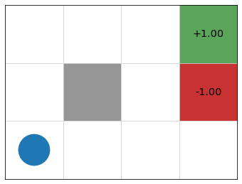
states = cells
actions = up, down, left, right, 10% chance of 90$\degree$ error
reward $r(s) = 0$ for non-terminal nodes
discount factor $\gamma = 0.9$

Value Function

A value function $V(s)$ is a prediction of future reward attainable starting from state $s$. \[ \begin{align} V(s) &= \max_{a \in A(s)} Q(s, a) \\ &= \max_a \mathbb{E}[R_{t+1} + \gamma R_{t+2} + \gamma^2 R_{t+3} + \ldots | S_t = s, A_t = a] \end{align} \]

Idea: lets us evaluate a state as good/bad (according to long term reward potential), and choose actions likely to take us to “better” states.

Model

A model predicts what the environment will do next

$\mathcal{P}$ predicts the probability of the next state

$\mathcal{R}$ predicts the expectation of the next reward, e.g.

\[ \mathcal{P}^a_{ss'} = \mathbb{P}[S_{t+1} = s' | S_t = s, A_t = a] \]

\[ \mathcal{R}^a_s = \mathbb{E}[R_{t+1} | S_t = s, A_t = a] \]

More “expensive” than learning value function or policy, which compress this info into “what I actually care about” and “what I should do”.

Categorizing RL methods

Value Based

No Policy (Implicit)
Value Function

Policy Based

Policy
No Value Function

Actor Critic

Policy
Value Function

Model Free

Policy and/or Value Function
No Model

Model Based

Policy and/or Value Function
Model

Value Iteration

The Bellman Equation

Value Iteration uses dynamic programming to recursively calculate a value function from an MDP.

\[ V(s) = \overbrace{\max_{a \in A(s)}}^{\text{best action from $s$}} \overbrace{\underbrace{\sum_{s' \in S}}_{\text{for every state}} P_a(s' \mid s) [\underbrace{R(s,a,s')}_{\text{(est. of) immediate reward}} + \underbrace{\gamma}_{\text{discount factor}} \cdot \underbrace{V(s')}_{\text{value of } s'}]}^{\text{expected reward $Q(s, a)$ of executing action $a$ in state $s$}} \]

Note: value iteration is model-based because it explicitly uses probability and reward distributions in calculation.

Calculating $V(s)$ by recursion

$V_0(s) = 0$ for all states $s$

$V_{i+1}(s) = \max\limits_{a \in A(s)} \sum\limits_{s' \in S} P_a(s' \mid s) [R(s, a, s') + \gamma V_i(s')]$

Example: GridWorld

\[ V_1(s) = \max\limits_{a \in A(s)} \sum\limits_{s' \in S} P_a(s' \mid s) R(s) + \gamma \underbrace{V_0(s')}_{0}] \]

$V_0$

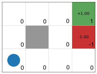
$V_1$

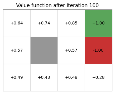
Example continued

\[ V_2(s) = \max\limits_{a \in A(s)} \sum\limits_{s' \in S} P_a(s' \mid s) [R(s) + \gamma V_1(s')] \]

$V_1$

$V_2$

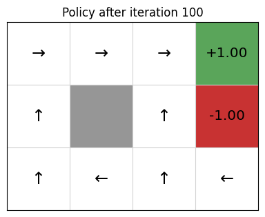
Policy Extraction

Once value function stabilizes, we extract a deterministic policy as

\[ \pi(s) = \text{argmax}_{a \in A(s)} \sum\limits_{s' \in S} P_a(s' \mid s)\ [R(s,a,s') + \gamma\ V(s')] \]

Monte Carlo Tree Search (MCTS)

Model-based methods

Replace real world with the agent’s (simulated) model of the environment
Supports rollouts (lookaheads) under imagined actions to reason about what value function will be, without further environment interaction

Model Learning

Goal: estimate model $\mathcal{M}_\eta$ from experience $\{S_1, A_1, R_2, \ldots, S_T\}$

This is a supervised learning problem

\[ \begin{aligned} S_1, A_1 &\;\to\; R_2, S_2 \\ S_2, A_2 &\;\to\; R_3, S_3 \\ &\;\vdots \\ S_{T-1}, A_{T-1} &\;\to\; R_T, S_T \end{aligned} \]

Learning $s,a \to r$ is a regression problem
Learning $s,a \to s'$ is a density estimation problem
Pick loss function, e.g. mean-squared error, KL divergence, …
Find parameters $\eta$ that minimise empirical loss

ExpectiMax Trees

Monte Carlo Tree search (MCTS) is based on representing MDPs as ExpectiMax trees that unfold as agents take actions.

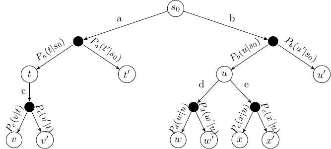
Note: state nodes are full histories

MCTS

Simultaneously “build” tree and maintain estimates of $Q(s,a)$ by simulating trajectories and observing rewards
Focus search on promising (as indicated by $Q$) states when state space is too large for value iteration
Maintain visit count $N(s)$ for states to inform strategy

MCTS Algoirithm

Starting from root node, successively select child nodes until leaf is reached.
Expand children by choosing action and creating new nodes based on possible outcomes.
Simulate trajectory from one of these nodes by choosing actions either at random or with heuristic
Backpropagate the total reward to prior nodes using Bellman equation to update $Q(a, s)$.

Multi-armed Bandits

Framework for selection strategy balancing exploration and exploitation

Multi-armed bandits

Intuition: For every state $s$, each action $a$ = slot machine with initually unknown payoff distributions $X_{a}$.

The “value” $Q(s, a)$ of $a$ corresponds to (current estimate of) $X_{a}$.

\[ Q_t(a, s) = \frac{R(a, t)}{N(a,s, t)} \]

where $N(a, s, t) =$ the number of times action $a$ has been performed in state $s$ at time $t$, and $R(a, t)$ is the total reward earned from those actions as of time $t$.

Bandit algorithm

Input: Multi-armed bandit problem $M = \langle a_i \sim X_i \rangle$

Output: $Q$-values $Q(a_i)$

$Q(a_i) \leftarrow 0$ for all arms $a_i$
$N(a_i) \leftarrow 0$ for all arms $a_i$
$t \leftarrow 1$

while $t < T$ do

$a \leftarrow$ select($k$)
execute arm $a$ for round $k$ and observe reward $r(a, t)$
$N(a) \leftarrow N(a) + 1$
$Q(a) \leftarrow Q(a) + \frac{1}{N(a)}[r(a, t) 0 Q(a)]$
$t \leftarrow t+1$

Bandit Selection Rules

$\epsilon$-first
$\epsilon$-greedy
$\epsilon$-decreasing
Upper confidence bound (UCB)
softmax

$\epsilon$-first

Perform random actions for $\epsilon*T$ rounds, where $T =$ total number of rounds.

For each strategy, consider:

What do the parameeters mean for us as modelers?
What does it mean for these numbers to be bigger/smaller?
What are the benefits and pitfalls of each strategy?
In what situations might we choose a particular strategy with particular parameter values?

$\epsilon$-greedy

with probability $1 - \epsilon$, choose the arm with maximum $Q$-value (exploit)
with probability $\epsilon$, choose arm uniformly at random (explore)

$\epsilon$-decreasing

Adds a variable $\alpha$ = “decay”
Like $\epsilon$ greedy, but explore probability is $\epsilon*\alpha^t$ at timestep $t$

UCB1 (Upper confidence bound)

\[ \text{argmax}_{a}\Bigl( \overbrace{Q_t(a)}^{\text{exploit best action}} + \underbrace{\sqrt{\frac{2 \ln t}{N_t(a)}}}_{\text{explore to reduce ``UCB" on alternatives}}\Bigr) \]

Based on Hoeffding’s inequality in probability theory, moderates “greediness” based on the likely accuracy of estimate of $Q(a)$ given available data
UCB “exploration bonus” term grows slowly (logarithmically) with $t$, but shrinks with larger sample size $N_t(a)$.

softmax

\[ P(a) = \frac{e^{Q(a)/\tau}}{\sum_{b\in A} e^{Q(b)/\tau}} \]

Approximates ratio of (exponential funciton of) current expected return for $a$ compared to alternatives

$\tau$ $\geq 0$ is the temperature parameter. Dictates influence of current value of $Q$ on decision.

lower $\tau$ = more exploitation: small differences in $Q$ get amplified in exponent, approaching argmax as $\tau \to 0^+$.
higher $\tau$ = more exploration: approaches uniform random as $\tau \to \infty$.

softmax continued

Softmax works well under drift– when underlying reward distributons change over time
Graph shows softmax performance for “restless bandit” where reward distributions abruptly change at $t= 250$.

Comparing bandit strategies

no drift

drift

Upper Confidence Trees (UCT)

MCTS commonly uses a variant of UCB for its selection rule:

\[ \text{argmax}_{a \in A(s)} \Bigl( Q(s, a) + \alpha\sqrt{\frac{2 \ln(N(s))}{N(s, a)}} \Bigr) \]

where $N(s)$ is the number of times a node has been visited, $N(s, a)$ is the number of times action $a$ has been chosen in that state, and $\alpha$ is an exploration parameter.

Note: when $N(a) = 0$, second term is “infinity”, i.e., always choose unexplored actions first.