04 Delete Relaxation

Motivation

Introduction to Relaxation

Delete relaxation is a method to relax planning tasks and automatically compute a heuristic function \(h\)

Delete relaxation is a widely used heuristic, highly successful for satisficing planning
Note that every \(h\) function typically yields good performance in only in some domains (balancing search reduction versus computational overhead).
- Therefore we aim for multiple alternative relaxation methods, depending upon domain

Relaxation Types

Four known types of relaxation that generate heuristics include

Critical path heuristics
Delete relaxation (covered in this Module)
Abstractions
Landmarks

Relaxing the World by Ignoring Delete Lists

“What was once true remains true forever”

The Delete Relaxation

Definition: The Delete Relaxation

We denote a STRIPS action \(a^+\), corresponding to \(a\), as the delete relaxed action (or just relaxed action), defined by \(pre_{a^+}:= pre_a\), \(\;add_{a^+}:= add_a\), and \({\color{blue}\;del_{a^+}:=}\) \({\color{blue}\emptyset}\)
A set of actions \(A^+\) corresponds to a set of relaxed actions \(A^+ := \{a^+ \mid a \in A\}\); and for a sequence of actions \(\vec{a} = \langle a_1, \dots, a_n\rangle\) denoted by \(\vec{a}^+\), we denote the corresponding sequence of relaxed actions as \(\vec{a}^+ := \langle a_1^+, \dots, a_n^+\rangle\).
For STRIPS planning task \(\Pi=(F,A,c,I,G)\) we denote the relaxed planning task as \(\Pi^+ := (F,A^+,c,I,G)\).

The “\(^+\)” super-script denotes delete relaxed states encountered in the relaxed version of the problem, e.g. \(s^+\) is a fact set just like \(s\).

The “\(^+\)” symbol is chosen to capture the additive (monotone) aspect of delete relaxed planning problems.

The Relaxed Plan

Definition: The Relaxed Plan

Let \(\Pi=(F,A,c,I,G)\) be a STRIPS planning task, and let \(s\) be a state.

An optimal relaxed plan for \({\color{red}s}\) is an optimal plan for \({\color{red}\Pi_s^+}\).
A relaxed plan for \(I\) is also called a relaxed plan for \(\Pi\).

Question: Do you recall what \(\Pi_s\) is?:

\(\Pi_s = (F,A,c,{\color{red}s},G)\)

A Relaxed Plan for “TSP” in Australia

Initial state: \(\{\mathit{at}(\mathit{Sy}), \mathit{v}(\mathit{Sy})\}\)
Apply \(\mathit{drive}(\mathit{Sy},\mathit{Br})^+\): \(\{\mathit{at}(\mathit{Br}), \mathit{v}(\mathit{Br}),\) \(\mathit{at}(\mathit{Sy}), \mathit{v}(\mathit{Sy})\}\)
Apply \(\mathit{drive}(\mathit{Sy},\mathit{Ad})^+\): \(\{\mathit{at}(\mathit{Ad}), \mathit{v}(\mathit{Ad}),\) \(\mathit{at}(\mathit{Br}), \mathit{v}(\mathit{Br}),\) \(\mathit{at}(\mathit{Sy}), \mathit{v}(\mathit{Sy})\}\)
Apply \(\mathit{drive}(\mathit{Ad},\mathit{Pe})^+\): \(\{\mathit{at}(\mathit{Pe}), \mathit{v}(\mathit{Pe}),\) \(\mathit{at}(\mathit{Ad}), \mathit{v}(\mathit{Ad}),\) \(\mathit{at}(\mathit{Br}), \mathit{v}(\mathit{Br}),\) \(\mathit{at}(\mathit{Sy}), \mathit{v}(\mathit{Sy})\}\)
Apply \(\mathit{drive}(\mathit{Ad},\mathit{Da})^+\): \(\{\mathit{at}(\mathit{Da}), \mathit{v}(\mathit{Da}),\) \(\mathit{at}(\mathit{Pe}), \mathit{v}(\mathit{Pe}),\) \(\mathit{at}(\mathit{Ad}), \mathit{v}(\mathit{Ad}),\) \(\mathit{at}(\mathit{Br}), \mathit{v}(\mathit{Br}),\) \(\mathit{at}(\mathit{Sy}), \mathit{v}(\mathit{Sy})\}\)

State Dominance

Definition of State Dominance

Definition: State Dominance

Let \(\Pi^+=(F,A^+,c,I,G)\) be a STRIPS planning task, and let \(s^+\) and \(s^{\prime +}\) be states, we say that state \(s^{\prime +}\) dominates state \(s^+\) if \(s^{\prime +} \supseteq s^+\) (every fact true in \(s^+\) is also true in \(s^{\prime +}\)).

For example, on the previous slide, what state dominates what? Each state along the relaxed plan dominates the previous one, because the actions don’t delete any facts.

Proposition: State Dominance Properties

Let \(\Pi^+=(F,A^+,c,I,G)\) be a delete relaxed STRIPS planning task, and let \(s^+\) and \(s^{\prime +}\) be states such that \(s^{\prime +}\) dominates \(s^+\).

If \(s^+\) is a goal state, then \(s^{\prime +}\) is also a goal state.
If an action sequence \(\vec a^+\) is applicable in \(s^+\) (i.e. \(pre(a^+) \subseteq s^+\) for all \(a^+ \in \vec a^+\)), then it is also applicable in \(s^{\prime +}\), and the state resulting from applying \(\vec a^+\) in \(s^{\prime +}\) denoted \(appl(s^{\prime +} \vec a^+)\), dominates the state resulting from applying \(\vec a^+\) in \(s^+\), \(appl(s^+, \vec a^+)\).

Proof: (i) is trivial. (ii) by induction over the length \(n\) of \(\vec{a}^+\). The base case \(n=0\) is trivial. The inductive case \(n \rightarrow n+1\) follows directly from the induction hypothesis and the definition of \(appl(.,.)\). In a delete=relaxed setting it is always better to have more facts true.

The Delete Relaxation & Admissibility

Proposition: Action Dominance

Let \(\Pi=(F,A,c,I,G)\) be a STRIPS planning task, let \(s\) be a state, and let \(a \in A\), then \(appl(s,a^+)\) dominates facts from both (i) \(s\), and (ii) \(appl(s,a)\).

Proof. Trivial from the definitions of \(appl(s,a)\) and \(a^+\).

Proposition: Delete Relaxation is Admissible

Let \(\Pi=(F,A,c,I,G)\) be a STRIPS planning task, let \(s\) be a state, and let \(\vec{a}\) be a plan for \(\Pi_s\). Then \(\vec{a}^+\) is a relaxed plan for \(\Pi_s^+\).

Optimal relaxed plans admissibly estimate the cost of optimal plans

Applying a relaxed action can only ever make more facts true ((i) from Action Dominance proposition above).
this can only be good, i.e. it cannot render a task unsolvable (dominance proposition)
It also means the relaxed plan can only be shorter, and hence is an (admissible) bound on how good the optimal plan could be (never over-estimates).

Proof: Prove by induction over the length of \(\vec{a}\) that \(appl(s,\vec{a}^+)\) dominates \(appl(s,\vec{a})\). Base case is trivial, inductive case follows from (ii) above.

Can you think of a method (greedy is OK) to find a relaxed plan?: We could keep applying relaxed actions, and only stop if the goal is true.

Relaxed Planning Methods

Greedy Relaxed Planning

Greedy Relaxed Planning for \(\Pi^+_s\)

\(s^+ := s\); \(\vec{a}^+ := \langle \rangle\)
while \(G \not \subseteq s^+\) do:
     if \(\exists a \in A\) such that \(pre_a \subseteq s^+\) and \(appl(s^+,a^+) \neq s^+\) then
         select one such \(a\)
         \(s^+ := appl(s^+,a^+)\); \(\vec{a}^+ := \vec{a}^+ \circ \langle a^+ \rangle\)
     else return “\(\Pi_s^+\) is unsolvable” endif
endwhile
return \(\vec{a}^+\)

Proposition Greedy relaxed planning is sound, complete, and terminates in time polynomial in the size of \(\Pi\).

Proof: Soundness: If \(\vec{a}^+\) is returned then, by construction, \(G \subseteq appl(s,\vec{a}^+)\). Completeness: If “\(\Pi_s^+\) is unsolvable” is returned, then no relaxed plan exists for \(s^+\) at that point; since \(s^+\) dominates \(s\), by the dominance proposition this implies that no relaxed plan can exist for \(s\). Termination: Every \(a \in A\) can be selected at most once because afterwards \(appl(s^+,a^+) = s^+\).

It is easy to decide whether a relaxed plan exists!

Greedy Relaxed Planning to Generate a Heuristic Function?

Using greedy relaxed planning to generate \(h\)

In search state \(s\) during forward search, run greedy relaxed planning on \(\Pi_s^+\).
Set \(h(s)\) to the cost of \(\vec{a}^+\), or \(\infty\) if “\(\Pi_s^+\) is unsolvable” is returned.

Is this heuristic safe?:

Yes: \(h(s)=\infty\) only if no relaxed plan for \(s\) exists, which by admissibility of delete relaxation implies that no plan for \(s\) exists.

Is this heuristic goal-aware?

Yes, we’ll have \(G \subseteq s^+\) right at the start.

Is this heuristic admissible?

No. It would be if relaxed plans were optimal; but clearly aren’t. So \(h\) isn’t consistent either.

To be informed (accurately estimate \(h^*\)), a heuristic must approximate the minimum effort needed to reach the goal. Greedy relaxed planning cannot be guaranteed to use minimum effort because it may select arbitrary actions that aren’t relevant at all.

\(h^+\): The Optimal Delete Relaxation Heuristic

Definition: \(h^+\)

Let \(\Pi=(F,A,c,I,G)\) be a STRIPS planning task with state space \(\Theta_\Pi=(S,A,c,T,I,G)\). The optimal delete relaxation heuristic \(h^+\) for \(\Pi\) is the function \(h^+ : S \mapsto \mathbb{R}_0^+ \cup \{\infty\}\) where \(h^+(s)\) is defined as the cost of an optimal relaxed plan for \(s\).

Corollary: \(h^+\) is Admissible

Let \(\Pi=(F,A,c,I,G)\) be a STRIPS planning task. Then \(h^+\) is admissible, and thus safe and goal-aware.

\(h^+\) naturally approximates the minimum effort by asking for the cheapest possible relaxed plans.

You might rightfully ask: But won’t optimal relaxed plans usually under-estimate \(h^*\)?

Yes, but that is just the definition of admissibility in the relaxed problem: it must never over estimates the true cost of the problem.
Arbitrarily adding actions greedily that are useless within the relaxation does not help to address it.

\(h^+\) in the TSP: Difference between \(h^*\) and \(h^+\)

\(P\): \(\mathit{at}(X)\) for \(X \in \{\mathit{Sy}, \mathit{Ad}, \mathit{Br}, \mathit{Pe}, \mathit{Ad}\}\); \(\mathit{v}(X)\) for \(X \in \{\mathit{Sy}, \mathit{Ad}, \mathit{Br}, \mathit{Pe}, \mathit{Ad}\}\).
\(A\): \(\mathit{drive}(X,Y)\) where \(X,Y\) have a road. \[ c(\mathit{drive}(X,Y)) = \left \{ \begin{array}[]{ll} 1 & \{X,Y\} = \{\mathit{Sy}, \mathit{Br}\}\\ 1.5 & \{X,Y\} = \{\mathit{Sy}, \mathit{Ad}\}\\ 3.5 & \{X,Y\} = \{\mathit{Ad}, \mathit{Pe}\}\\ 4 & \{X,Y\} = \{\mathit{Ad}, \mathit{Da}\} \end{array} \right. \]
\(I\): \(\mathit{at}(\mathit{Sy}), \mathit{v}(\mathit{Sy})\); \(G\): \(\mathit{at}(\mathit{Sy}), \mathit{v}(X) \text{ for all } X\).

Planning versus Relaxed Planning:

Optimal plan: \(\langle \mathit{drive}(\mathit{Sy},\mathit{Br})\), \(\mathit{drive}(\mathit{Br},\mathit{Sy})\), \(\mathit{drive}(\mathit{Sy},\mathit{Ad})\), \(\mathit{drive}(\mathit{Ad},\mathit{Pe})\), \(\mathit{drive}(\mathit{Pe},\mathit{Ad})\), \(\mathit{drive}(\mathit{Ad},\mathit{Da})\), \(\mathit{drive}(\mathit{Da},\mathit{Ad})\), \(\mathit{drive}(\mathit{Ad},\mathit{Sy}) \rangle\).
Optimal relaxed plan: \(\langle \mathit{drive}(\mathit{Sy},\mathit{Br})\), \(\mathit{drive}(\mathit{Sy},\mathit{Ad})\), \(\mathit{drive}(\mathit{Ad},\mathit{Pe})\), \(\mathit{drive}(\mathit{Ad},\mathit{Da}) \rangle\).
\({\color{blue}h^{*}(I)=}\) \(20\); \({\color{blue}h^+(I)=}\) \(10\).

\(h^+\) in the TSP: What problem does this remind you of?

Towers of Hanoi: \(h^+\) can underestimate a lot!

\(h^+\)(Hanoi) \(= O(n)\), as opposed to problem complexity of \(O(2^n)\) (the shortest plan which solves the problem can be exponential)

But how do we Compute \(h^+\)?

Definition: Optimal Relaxed Planning

By PlanOpt\(^+\), we denote the problem of deciding, given a STRIPS planning task \(\Pi = (F,A,c,I,G)\) and \(B \in \mathbb{R}^+_0\), whether there exists a relaxed plan for \(\Pi\) whose cost is at most \(B\).

Note. By computing \(h^+\), we would solve PlanOpt\(^+\).

Theorem: Optimal Relaxed Planning is Hard

Theorem: Optimal Relaxed Planning is Hard.

PlanOpt\(^+\) is NP-complete.

Proof. Membership: Guess action sequences of length \(|A|\) — in a relaxed plan, each action is applied at most once!

Hardness: by reduction from SAT.

For each variable \(v_i \in \{v_1, \dots, v_m\}\) in the CNF, three facts \(\mathit{v}_i\), \(\mathit{notv}_i\), and \(\mathit{setv}_i\); for each clause \(c_j \in \{c_1, \dots, c_n\}\) in the CNF, one fact \(\mathit{satc}_j\).
Actions {\(\mathit{setvtrue}_i : (\emptyset,\{\mathit{v}_i,\mathit{setv}_i\},\emptyset)\)} and {\(\mathit{setvfalse}_i : (\emptyset,\{\mathit{notv}_i,\mathit{setv}_i\},\emptyset)\)}.
Actions {\(\mathit{makesatc}_j : (\{\mathit{v}_i\},\{\mathit{satc}_j\},\emptyset)\)} where \(v_i\) appears positively in clause \(c_j\); and {\((\{\mathit{notv}_i\},\{\mathit{satc}_j\},\emptyset)\)} where \(v_i\) appears negatively in clause \(c_j\).
Initial state \(\emptyset\), goal \(\{\mathit{setv}_1, \dots, \mathit{setv}_m, \mathit{satc}_1, \dots, \mathit{satc}_n\}\); {\(B := m+n\)}.

\(h^+\) as a Relaxation Heuristic for STRIPS Planning tasks

where, for all \(\Pi \in \mathcal P\), \(h^*(r(\Pi)) \leq h^*(\Pi)\).

For \(h^+ = h^* \circ r\):

Problem \(\mathcal P\): All STRIPS planning tasks.
Simpler problem \(\mathcal P'\): All STRIPS planning tasks with empty deletes.
Perfect heuristic \(h^{\prime *}\) for \(\mathcal P'\): Optimal plan cost \(= h^*\) on \(\mathcal P'\).
Transformation \(r\): Drop the deletes.

Is this a native relaxation? Yes.

Is this relaxation efficiently constructible? Yes.

Is this relaxation efficiently computable? No.

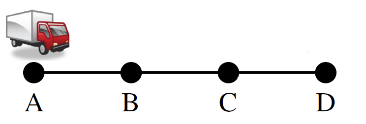
How to Relax if not efficiently computable? Approximate

Reminder: What if \(\mathcal R\) is not efficiently computable?

Either (a) approximate \(h^{\prime *}\), or (b) design \(h^{\prime *}\) in a way so that it will typically be feasible, or (c) just live with it and hope for the best.
Many known relaxations (in planning) are efficiently computable, some aren’t (like \(h^+\)). The latter use (a); (b) and (c) are not used anywhere right now.

The delete relaxation heuristic we want is \(h^+\).

Unfortunately, this is hard to compute so the computational overhead is very likely to be prohibitive.

All implemented systems are using the delete relaxation approximate \(h^+\) in one or the other way.

We now look at the the most wide-spread approaches to do so.

Indiana Jones’ Maze Domain?

Question

In this domain, what is the delete relaxed heuristic \(h^+\) equal to?

(A) Manhattan distance.

(B) \(h^*\).

(D) Vertical distance.

(A): No, relaxed plans can’t walk through walls.

(B): Yes, optimal plan = shortest path = relaxed plan (deletes do not matter because “shortest paths never walk back”).

(C), (D): No, relaxed plans must move both horizontally and vertically.

The Additive and Max Heuristics

The Additive Heuristics

Definition: \(h^{add}\)

Let \(\Pi=(F,A,c,I,G)\) be a STRIPS planning task. The additive heuristic \({\color{blue}h^{add}}\) for \(\Pi\) is the function \(h^{add}(s) := h^{add}(s,G)\) where \(h^{add}(s,g)\) is the point-wise greatest function that satisfies

\[ \color{blue} h^{add}(s,g) = \left \{ \begin{array}[]{ll} 0 & g \subseteq s\\ min_{a \in A, g \in add_a} c(a) + h^{add}(s,pre_a) & |g| = 1\\ {\color{red}\sum_{g' \in g}} h^{add}(s,\{g'\}) & |g| > 1 \end{array} \right. \]

The Max Heuristics

Definition: \(h^{max}\)

Let \(\Pi=(F,A,c,I,G)\) be a STRIPS planning task. The max heuristic \({\color{blue}h^{max}}\) for \(\Pi\) is the function \(h^{max}(s) := h^{max}(s,G)\) where \(h^{max}(s,g)\) is the point-wise greatest function that satisfies

\[ \color{blue} h^{max}(s,g) = \left \{ \begin{array}[]{ll} 0 & g \subseteq s\\ min_{a \in A, g \in add_a} c(a) + h^{max}(s,pre_a) & |g| = 1\\ {\color{red}\max_{g' \in g}} h^{max}(s,\{g'\}) & |g| > 1 \end{array} \right. \]

The Additive and Max Heuristics: Properties

Proposition: \(h^{max}\) is Optimistic

\(h^{max} \leq h^+\), and thus \(h^{max} \leq h^*\).

Proposition: \(h^{add}\) is Pessimistic

For all STRIPS planning tasks \(\Pi\), \(h^{add} \geq h^+\), there exist \(\Pi\) and \(s\) such that \(h^{add}(s) > h^*(s)\).

Both \(h^{max}\) and \(h^{add}\) approximate \(h^{add}\) by assuming that singleton sub-goal facts are achieved independently.

\({\color{blue}h^{max}}\) estimates optimistically by the most costly singleton sub-goal
\({\color{blue}h^{add}}\) estimates pessimistically by summing over all singleton sub-goals

The Additive and Max Heuristics: Properties (Continued)

Proposition: \(h^{max}\) and \(h^{add}\) Agree with \(h^+\) on \(\infty\)

For all STRIPS planning tasks \(\Pi\) and states \(s\) in \(\Pi\), \(h^+(s) = \infty\) if and only if \(h^{max}(s) = \infty\) if and only if \(h^{add}(s) = \infty\).

States for which no relaxed plan exists are easy to recognise, and that is done by both \(h^{max}\) and \(h^{add}\).

Approximation is needed only for the cost of an optimal relaxed pan, if it exists.

Bellman-Ford: Fixed Point Iterative Algorithm for \(h^{add}\)

Bellman-Ford variant computing \(h^{add}\) for state \(s\)

Create a new table \(T^{\text{\textup{add}}}_{0}(g)\), for \(g \in F\)
For all \(g \in F: T^{\text{\textup{add}}}_{0}(g) := \left \{ \begin{array}[]{ll} 0 & g \in s \\ \infty & \text{otherwise}\end{array} \right.\)
fn \(c_i(g) := \left \{ \begin{array}[]{ll} T^{\text{\textup{add}}}_{i}(g) & |g| = 1\\ {\color{blue}\sum}_{g' \in g} T^{\text{\textup{add}}}_{i}(g') & |g| > 1 \end{array}\right.\)
fn \(f_i(g) := \min[c_i(g), \min_{a \in A, g \in add_a} c(a) + c_i(pre_a)]\)
do = forever:
           new table \(T^{\text{\textup{add}}}_{i+1}(g)\), for \(g \in F\)
           For all \(g \in F\): \(T^{\text{\textup{add}}}_{i+1}(g) := f_i(g)\)
           if \(T^{\text{\textup{add}}}_{i+1} = T^{\text{\textup{add}}}_{i}\) then stop endif /* least fixed point achieved, so stop */
           \(i\) := \(i+1\)
enddo

The same algorithm works for \(h^{max}\) as well, just change \({\color{blue}\sum}\) to \({\color{blue}max}\)

Bellman-Ford Convergence for \(h^{add}\)

Proposition: Convergence

Let \(\Pi=(F,A,c,I,G)\) be a STRIPS planning task, then the series \(\{T^{\text{\textup{add}}}_i(g)\}_{i=0, \dots}\) converges to \(h^{add}(s,g)\), for all \(g\). (Proof omitted.)

Bellman-Ford for \(h^{max}\) in TSP Example?

\(P\): \(\mathit{at}(X)\) for \(X \in \{\mathit{Sy}, \mathit{Ad}, \mathit{Br}, \mathit{Pe}, \mathit{Ad}\}\); \(\mathit{v}(X)\) for \(X \in \{\mathit{Sy}, \mathit{Ad}, \mathit{Br}, \mathit{Pe}, \mathit{Ad}\}\).
\(A\): \(\mathit{drive}(X,Y)\) where \(X,Y\) have a road. \[ c(\mathit{drive}(X,Y)) = \left \{ \begin{array}[]{ll} 1 & \{X,Y\} = \{\mathit{Sy}, \mathit{Br}\}\\ 1.5 & \{X,Y\} = \{\mathit{Sy}, \mathit{Ad}\}\\ 3.5 & \{X,Y\} = \{\mathit{Ad}, \mathit{Pe}\}\\ 4 & \{X,Y\} = \{\mathit{Ad}, \mathit{Da}\} \end{array} \right. \]
\(I\): \(\mathit{at}(\mathit{Sy}), \mathit{v}(\mathit{Sy})\); \(G\): \(\mathit{at}(\mathit{Sy}), \mathit{v}(X) \text{ for all } X\).

Content of Tables \(T^{add}_i\)?: where \(T^{add}_i\) denotes table entry after \(i\)-th Bellman-Ford iteration?

\({\color{red}h^{max}(I)=}\) \(5.5 << 20 = h^*(I)\).

Bellman-Ford for \(h^{add}\) in TSP Example?

\(P\): \(\mathit{at}(X)\) for \(X \in \{\mathit{Sy}, \mathit{Ad}, \mathit{Br}, \mathit{Pe}, \mathit{Ad}\}\); \(\mathit{v}(X)\) for \(X \in \{\mathit{Sy}, \mathit{Ad}, \mathit{Br}, \mathit{Pe}, \mathit{Ad}\}\).
\(A\): \(\mathit{drive}(X,Y)\) where \(X,Y\) have a road. \[ c(\mathit{drive}(X,Y)) = \left \{ \begin{array}[]{ll} 1 & \{X,Y\} = \{\mathit{Sy}, \mathit{Br}\}\\ 1.5 & \{X,Y\} = \{\mathit{Sy}, \mathit{Ad}\}\\ 3.5 & \{X,Y\} = \{\mathit{Ad}, \mathit{Pe}\}\\ 4 & \{X,Y\} = \{\mathit{Ad}, \mathit{Da}\} \end{array} \right. \]
\(I\): \(\mathit{at}(\mathit{Sy}), \mathit{v}(\mathit{Sy})\); \(G\): \(\mathit{at}(\mathit{Sy}), \mathit{v}(X) \text{ for all } X\).

Content of Tables \(T^{add}_i\)?: where \(T^{add}_i\) denotes table entry after \(i\)-th Bellman-Ford iteration?

\({\color{red}h^{add}(I)=}\) \(1.5 + 1 + 5 + 5.5 = 13 > 10 = h^+(I)\). But \(< 20 = h^*(I)\).

\(h^{add}(I) > h^+(I)\) because it counts the cost of \(\mathit{drive}(\mathit{Sy},\mathit{Ad})\) 3 times:

As part of \(h^{add}(I,\{\mathit{v}(\mathit{Ad})\})\), \(h^{add}(I,\{\mathit{v}(\mathit{Pe})\})\), and \(h^{add}(I,\{\mathit{v}(\mathit{Da})\})\)!

Difference between \(h^{add}\) & \(h^{max}\) in Logistics?

Initial state \(I\): \(t(A), p(C)\)
Goal \(G\): \(t(A), p(D)\)
Actions \(A\): dr(X,Y), lo(X), ul(X).

Content of Tables ?: \(T^{add}_i\) entries are denoted in black and \({\color{red}T^{max}_i}\) in red.

\({\color{red} h^{add}(I)=}\) \(7 > h^+(I) = 5\), but \(< 8 = h^*(I)\).

\(h^{add}(I) > h^+(I)\) because? It counts the cost of \(\mathit{dr}(A,B), \mathit{dr}(B,C)\) 2 times, for the two preconditions \(\mathit{p}(T)\) and \(\mathit{t}(D)\) of achieving \(\mathit{p}(D)\).

So, what if \(G = \{\mathit{t}(D), \mathit{p}(D)\}\)? \(h^{add}(I)=\) \(10 > 5 = h^*(I) = h^+(I)\) because now \(\mathit{dr}(A,B), \mathit{dr}(B,C), \mathit{dr}(C,D)\) is counted also as part of the goal \(\mathit{t}(D)\).

The Additive and Max Heuristics in Practice?

Summary of typical issues in practice with \(h^{add}\) and \(h^{max}\):

Both \(h^{add}\) and \(h^{max}\) can be used to approximate \(h^+\) and can be computed reasonably quickly.
\(h^{max}\) is admissible, but is typically far too optimistic.
\(h^{add}\) is not admissible as it is pessimistic, but is typically a lot more informed than \(h^{max}\).
\(h^{add}\) is sometimes better informed than \(h^+\), but can be for the wrong reasons: rather than accounting for deletes, it overcounts by ignoring positive interactions, i.e. sub-plans shared between sub-goals.
- Such overcounting can result in large over-estimates of \(h^\ast\).

For the Logistics example above with goal \(\mathit{t}(d)\), if we have \(100\) packages at \(c\) that need to go to \(d\), what is \(h^{add}(I)\)?

\(703 \gg 203 = h^\ast(I) = h^+(I)\): For every package, a count of \(7\) which includes \(\mathit{dr}(a,b), \mathit{dr}(b,c)\) for getting the package into the truck, and \(\mathit{dr}(a,b), \mathit{dr}(b,c), \mathit{dr}(c,d)\) for getting the truck to \(d\).

Relaxed plans (up next) are a means to reduce this kind of over-counting.

Relaxed Plans

Best Supporter Function

First compute a best-supporter function \(bs\), which for every fact \(p \in F\) returns an action that is deemed to be the cheapest achiever of \(p\) (within the relaxation).
Then extract a relaxed plan from that function, by applying it to singleton sub-goals and collecting all the actions.

The best-supporter function can be based directly on \(h^{max}\) or \(h^{add}\), simply selecting an action \(a\) achieving \(p\) that minimizes the sum of \(c(a)\) and the cost estimate for \(pre_a\).

Best-Supporter Functions

Definition: Best-Supporters from \(h^{max}\) and \(h^{add}\)

Let \(\Pi=(F,A,c,I,G)\) be a STRIPS planning task, and let \(s\) be a state, and \(p\) be sub-goals, such that \(p \in G\).

The \(h^{max}\) supporter function \(bs^{max}_s : \{p \in F \mid 0 < h^{max}(s,\{p\}) < \infty\} \mapsto A\) is defined by \(bs^{max}_s(p) := \arg\min_{a \in A, p \in add_a} \Big( c(a) + h^{max}(s,pre_a)\Big).\)

The \({\color{blue}h^{add}}\) supporter function \(bs^{add}_s: \{p \in F \mid 0 < h^{add}(s,\{p\}) < \infty\} \mapsto A\) is defined by \({\color{red}bs^{add}_s(p) := \arg\min_{a \in A, p \in add_a} \Big( c(a) + h^{add}(s,pre_a)\Big)}\).

Example \(h^{add}\) in Logistics:

Relaxed Plan Extraction via Best Supporter Functions

Relaxed Plan Extraction for state \(s\) and best-supporter function \(bs\)

\(\mathit{Open} := G \setminus s\); \(\mathit{Closed} := \emptyset\); \(\mathit{RPlan} := \emptyset\)
while \(Open \neq \emptyset\) do:
      select \(g \in \mathit{Open}\)
      \(\mathit{Open} := \mathit{Open} \setminus \{g\}\); \(\mathit{Closed} := \mathit{Closed} \cup \{g\}\);
      \(\mathit{RPlan} := \mathit{RPlan} \cup \{{\color{red}bs(g)}\}\); \(\mathit{Open} := \mathit{Open} \cup (pre_{bs(g)} \setminus (s \cup \mathit{Closed}))\)
endwhile
return \(\mathit{RPlan}\)

Starting with top-level goals, iteratively close open singleton sub-goals by selecting best supporter. The number of iterations bounded by \(|P|\), however with the following requirements:

What if \(g \not \in add_{bs}(g)\)? Doesn’t make sense = requirement (A): \(\forall g, g \in add(bs(g))\), i.e. add effects must include goal

What if \(bs(g)\) is undefined? Runtime error = requirement (B): \(bs(g)\) must be defined

What if the support for \(g\) eventually requires \(g\) itself as a precondition? Then this does not actually yield a relaxed plan = requirement (C): must yield a relaxed plan

Relaxed Plan Extraction from \(h^{add}\) in Logistics?

Initial state \(I\): \(t(A), p(C)\)
Goal \(G\): \(t(A), p(D)\)
Actions \(A\): dr(X,Y), lo(X), ul(X).

Extracting a relaxed plan:

\(bs^{add}_s(\mathit{p}(D)) =\) \(\mathit{ul}(D)\); opens \(\mathit{t}(D), \mathit{p}(T)\).
\(bs^{add}_s(\mathit{t}(D)) =\) \(\mathit{dr}(C,D)\); opens\(\;\mathit{t}(C)\).
\(bs^{add}_s(\mathit{t}(C)) =\) \(\mathit{dr}(B,C)\); opens\(\;\mathit{t}(B)\).
\(bs^{add}_s(\mathit{t}(B)) =\) \(\mathit{dr}(A,B)\); opens nothing.
\(bs^{add}_s(\mathit{p}(T)) =\) \(\mathit{lo}(C)\); opens nothing.
Anything more? No, open goals empty at this point.

\({\color{red}\mathit{h^{\mathit{FF}}(I)=}}\) \(5 = h^+(I) < 7 = h^{add}(I) < 8 = h^*(I)\).

What if \(G = \{\mathit{t}(D), \mathit{p}(D)\}\)? \(h^{\mathit{FF}}(I)=\) \(5 = h^+(I) = h^*(I)\) because relaxed plan extraction selects the drive actions only once. By contrast, \(h^{add}(I) = 10\) overcounts these actions, c.f. Bellman-Ford for \(h^{add}\) in Logistics

Best-Supporter Functions

For relaxed plan extraction to make sense, it requires a best-supporter function

Definition: Best-Supporter Function

Let \(\Pi=(F,A,c,I,G)\) be a STRIPS planning task, and let \(s\) be a state. A best-supporter function for \(s\) is a partial function \(bs: (F \setminus s) \mapsto A\) such that \(p \in add_a\) whenever \(a = bs(p)\).

The support graph of \(bs\) is the directed graph with vertices \(F \cup A\) and arcs \(\{(p,a) \mid p \in pre_a\} \cup \{(a,p) \mid a = bs(p)\}\).

We say that \(bs\) is closed if \(bs(p)\) is defined for every \(p \in (F \setminus s)\) that has a path to a goal \(g \in G\) in the support graph.

We say that \(bs\) is well-founded if the support graph is acyclic.

“\(p \in add_a\) whenever \(a = bs(p)\)”: Requirement (A).
\(bs\) is closed: Requirement (B).
\(bs\) is well-founded: Requirement (C).

Intuition for (C): Relaxed plan extraction starts at the goals, and chains backwards in the support graph. If there are cycles, then this backchaining may not reach the currently true state \(s\), and thus not yield a relaxed plan.

Support Graphs and Prerequisite (C) in Logistics

Initial state: \(\mathit{t}A\).
Goal: \(\mathit{t}D\).
Actions: \(\mathit{dr}XY\).

How to do it (well-founded)

How NOT to do it (not well-founded)

The definition implies a closed, well-founded \(bs\)!

Definition (Revisited): Best-Supporters from \(h^{max}\) and \(h^{add}\)

Let \(\Pi=(F,A,c,I,G)\) be a STRIPS planning task, and let \(s\) be a state, and \(p\) be sub-goals, such that \(p \in G\).

The \(h^{max}\) supporter function \(bs^{max}_s : \{{\color{blue}p \in F \mid 0 < h^{max}(s,\{p\}) < \infty}\} \mapsto A\) is defined by \(bs^{max}_s(p) := \arg\min_{a \in A, p \in add_a} \Big( c(a) + h^{max}(s,pre_a)\Big).\)

The \(h^{add}\) supporter function \(bs^{add}_s: \{p \in F \mid 0 < h^{add}(s,\{p\}) < \infty\} \mapsto A\) is defined by \(bs^{add}_s(p) := \arg\min_{a \in A, p \in add_a} \Big( c(a) + h^{add}(s,pre_a)\Big)\).

Proposition

Let \(\Pi=(F,A,c,I,G)\) be a STRIPS planning task such that, for all \(a \in A\), \(c(a) > 0\). Let \(s\) be a state where \(h^+(s) < \infty\). Then both \(bs^{max}_s\) and \(bs^{add}_s\) are closed well-founded supporter functions for \(s\).

Proof. Since \(h^+(s) < \infty\) implies \(h^{max}(s) < \infty\), it is easy to see that \(bs^{max}_s\) is closed (details omitted).

If \(a = bs^{max}_s(p)\), then \(a\) is the action yielding \(0 < h^{max}(s,\{p\}) < \infty\) in the \(h^{max}\) equation.
Intuition: Since \(c(a) > 0\), we have \(h^{max}(s,pre_a) < h^{max}(s,\{p\})\) and thus, for all \(q \in pre_a\), \(h^{max}(s,\{q\}) < h^{max}(s,\{p\})\).
Transitively, if the support graph contains a path from fact vertex \(r\) to fact vertex \(t\), then \(h^{max}(s,\{r\}) < h^{max}(s,\{t\})\).
Thus there can’t be cycles in the support graph and \(bs^{max}_s\) is well-founded. Similar for \(bs^{add}_s\).

The Relaxed Plan Extraction: Correctness

Proposition

Let \(\Pi=(F,A,c,I,G)\) be a STRIPS planning task, let \(s\) be a state, and let \(bs\) be a closed well-founded best-supporter function for \(s\).

Then the action set \(\mathit{RPlan}\) returned by relaxed plan extraction can be sequenced into a relaxed plan \(\vec{a}^+\) for \(s\).

Proof. Order \(a\) before \(a'\) whenever the support graph contains a path from \(a\) to \(a'\). Since the support graph is acyclic, such a sequencing \(\vec{a} := \langle a_1, \dots, a_n \rangle\) exists.

We have \(p \in s\) for all \(p \in pre_{a_1}\), because otherwise \(\mathit{RPlan}\) would contain the action \(bs(p)\), necessarily ordered before \(a_1\).
We have \(p \in s \cup add_{a_1}\) for all \(p \in pre_{a_2}\), because otherwise \(\mathit{RPlan}\) would contain the action \(bs(p)\), necessarily ordered before \(a_2\). Iterating the argument shows that \(\vec{a}^+\) is a relaxed plan for \(s\).

The Relaxed Plan Heuristic: \(h^{FF}\)

Definition: Relaxed Plan Heuristic

A heuristic function is called a relaxed plan heuristic, denoted \({\color{blue}h^{\mathit{FF}}}\), if, given a state \(s\),

it returns \(\infty\) if no relaxed plan exists, and
otherwise returns \(\sum_{a \in \mathit{RPlan}} c(a)\) where \(\mathit{RPlan}\) is the action set returned by relaxed plan extraction on a closed well-founded best-supporter function for \(s\).

Recall if a relaxed plan exists, then there also exists a closed well-founded best-supporter function, see above.

By comparison:

\(h^{max}\) estimates by taking the hardest sub-goal
\(h^{add}\) estimates by summing sub-goal costs
\(h^{FF}\) estimates by extracting an actual relaxed plan in the delete-relaxed problem and then taking its cost.

The Relaxed Plan Heuristic (Continued)

Proposition: \(h^{\mathit{FF}}\) is Pessimistic and Agrees with \(h^*\) on \(\infty\)

For all STRIPS planning tasks \(\Pi\), \(h^{\mathit{FF}} \geq h^+\); for all states \(s\), \(h^+(s) = \infty\) if and only if \(h^{\mathit{FF}}(s) = \infty\). There exist \(\Pi\) and \(s\) so that \(h^{\mathit{FF}}(s) > h^*(s)\).

Proof. \(h^{\mathit{FF}} \geq h^+\) follows directly from the previous proposition. Agrees with \(h^+\) on \(\infty\): direct from definition. Inadmissiblity: Whenever \(bs\) makes sub-optimal choices. Exercise, perhaps

Relaxed plan heuristics have the same theoretical properties as \(h^{add}\).

So what’s the point?

Can \(h^{\mathit{FF}}\) over-count, i.e., count sub-plans shared between sub-goals more than once?

No, due to the set union in “\(\mathit{RPlan} := \mathit{RPlan} \cup \{\mathit{bs}(g)\}\)”.
\(h^{\mathit{FF}}\) be inadmissible, just like \(h^{add}\), but for more subtle reasons.
In practice, \(h^{\mathit{FF}}\) typically does not over-estimate \(h^*\) (or not by a large amount, anyway); example on previous “Logistics” slide.

Helpful Actions

Definition: Helpful Actions

Let \(h^{\mathit{FF}}\) be a relaxed plan heuristic, let \(s\) be a state, and let \(\mathit{RPlan}\) be the action set returned by relaxed plan extraction on the closed well-founded best-supporter function for \(s\) which underlies \(h^{\mathit{FF}}\).

Then an action \(a\) applicable to \(s\) is called helpful if it is contained in \(\mathit{RPlan}\).

Remarks

Initially introduced in FF [Hoffmann and Nebel (2011)], restricting Enforced Hill-Climbing to use only the helpful actions
Expanding only helpful actions does not guarantee completeness.
Other planners use helpful actions as preferred operators, first expanding nodes resulting from helpful actions.

Conclusion

Questions

Question

How does ignoring delete lists simplify FreeCell card game?

(A) You can move all cards immediately to their goal.

(B) Free cells remain free.

(A): No, we don’t get any new moves in the relaxation.

(B): Yes, when putting a card into a free cell, it’s still free for another card.

Questions (continued)

Question

How does ignoring delete lists simplify Sokoban game?

(A) Free positions remain free

(B) You can walk through walls

(D) Nothing ever becomes blocked

(A), (C), (D): Yes (similar to FreeCell)

(B): No, we don’t get any new moves

Summary

The delete relaxation simplifies STRIPS by removing all delete effects of the actions.
The cost of optimal relaxed plans yields the heuristic function \(h^+\), which is admissible but hard to compute.
We can approximate \(h^+\) optimistically by \(h^{max}\), and pessimistically by \(h^{add}\). \(h^{max}\) is admissible, \(h^{add}\) is not. \(h^{add}\) is typically much more informative, but can suffer from over-counting.
Either of \(h^{max}\) or \(h^{add}\) can be used to generate a closed well-founded best-supporter function, from which we can extract a relaxed plan. The resulting relaxed plan heuristic \(h^{\mathit{FF}}\) does not do over-counting, but otherwise has the same theoretical properties as \(h^{add}\); it typically does not over-estimate \(h^*\).

Example Classical Planning Systems

HSP [Bonet and Geffner, AI-01]

Search algorithm: Greedy best-first search.
Search control: \(h^{add}\).

FF [Hoffmann and Nebel, JAIR-01]

Search algorithm: Enforced hill-climbing.
Search control: \(h^{FF}\) extracted from the \(h^{max}\) supporter function; helpful actions pruning (basically expand only those actions contained in the relaxed plan).

LAMA [Richter and Westphal, JAIR-10]

Search algorithm: Multiple-queue greedy best-first search.
Search control: \(h^{FF}\) + a landmarks heuristic (similar to goal counting); for each, one search queue with all actions, one search queue with only helpful actions.

BFWS [Lipovetzky and Geffner, AAAI-17]

Search algorithm: Best-first width search.
Search control: Novelty + variant of \(h^{FF}\) + goal counting.

Remarks

The relaxation principle is a generic, widely applicable approach for many different contexts, as are other relaxation principles identified in the subject.

While the \(h^{max}\) heuristic is not very informative in practice, other lower-bounding approximations of \(h^+\) are very important for optimal planning, such as

Admissible landmarks heuristics [Karpas and Domshlak, IJCAI-09], and
LM-cut heuristic [Helmert and Domshlak, ICAPS-09].

It has always been a challenge to take some delete effects into account. Some work has been conducted to interpolate smoothly between \(h^+\) and \(h^*\), such as

Explicitly represented fact conjunctions [Keyder, Hoffmann, and Haslum ICAPS-12].

Advanced Reading

Planning as Heuristic Search [Bonet and Geffner, AI-01].

A paper charting the origins of heuristics search.
Available via Institutional Login: https://www.sciencedirect.com/science/article/pii/S0004370201001084

The FF Planning System: Fast Plan Generation Through Heuristic Search [Hoffmann:nebel:jair-01].

The main reference for delete relaxation heuristics.
Available for download at https://fai.cs.uni-saarland.de/hoffmann/papers/jair01.pdf

Advanced Reading (Continued)

Semi-Relaxed Plan Heuristics [Keyder, Hoffmann, and Haslum ICAPS-12].

Available at: http://fai.cs.uni-saarland.de/hoffmann/papers/icaps12a.pdf
Computes relaxed plan heuristics within a compiled planning task \(\Pi^C_{\mathit{ce}}\), in which a subset \(C\) of all fact conjunctions in the task is represented explicitly as suggested by [Haslum, ICAPS-12].
- \(C\) can in principle always be chosen so that \(h^+_{\Pi^{C}_{\mathit{ce}}}\) is perfect (equals \(h^*\) in the original planning task), so the technique allows to interpolate between \(h^+\) and \(h^*\).
- In practice, small sets \(C\) sometimes suffice to obtain dramatically more informed relaxed plan heuristics.