10 Policy Gradient (Actor Critic)

Table of contents

• Introduction
• Monte-Carlo Policy Gradient Methods
• Actor-Critic Methods

Introduction

Policy-Based Reinforcement Learning

In the last module we approximated the value or action-value function using parameters \(\theta\),

\[ \begin{align*} V_\theta(s) &\approx V^\pi(s) \\ Q_\theta(s, a) &\approx Q^\pi(s, a) \end{align*} \]

A policy was generated directly from the value function,
e.g. using \(\epsilon\)-greedy.

In this module we will directly parameterise a stochastic policy \(\textcolor{red}{\pi_\theta(a|s)}\) which tells us the probability of performing action \(a\) in state \(s\).

We will focus again on model-free reinforcement learning, and we directly change the probabilities we pick different actions

Value-Based and Policy-Based RL

Value Based

• Learnt Value Function

• Implicit policy (bandit strategy)

Policy Based

• No Value Function

• Learnt Policy

Actor-Critic

• Learnt Value Function

• Learnt Policy

Choice of value-function versus policy approximation sometimes depends on which is easier to compute and store according to the application

Advantages of Policy-Based RL

Advantages:

• Better convergence properties

• Effective in high-dimensional or continuous action spaces (as don’t need to estimate \(max\) directly, which can be expensive)

• Can learn stochastic policies

Disadvantages:

• Typically converges to a local rather than global optimum

• Evaluating a policy is typically inefficient and high variance

Example: Rock-Paper-Scissors

Two-player game of rock-paper-scissors

• Scissors beats paper

• Rock beats scissors

• Paper beats rock

A deterministic policy is easily exploited

• A uniform random policy is optimal (i.e. Nash equilibrium), i.e. optimal behaviour is stochastic

Example: Aliased Gridworld

The agent cannot differentiate the grey states (look the same), so agent policy must be the same in both states.

Question: Why is this a problem for deterministic policies? How can this problem be solved with a stochastic policy?

Example: Aliased Gridworld (2)

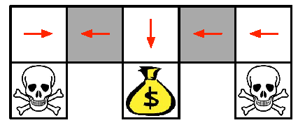
Under aliasing, an optimal deterministic policy will either

• move \(W\) in both grey states (shown by red arrows)

• move \(E\) in both grey states

Either way, it can get stuck and never reach the money

Value-based RL learns a near-deterministic policy

• e.g. greedy or \(\epsilon\)-greedy

So it will traverse the corridor for a long time

Example: Aliased Gridworld (3)

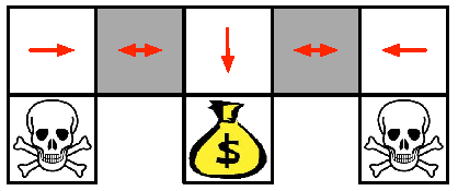
An optimal stochastic policy will randomly move \(E\) or \(W\) in grey states

\[ \begin{align*} \pi_{\theta}(\text{wall to}\;N \text{and}\;S, \text{move}\; E) & = 0:5\\[0pt] \pi_{\theta}(\text{wall to}\;N \text{and}\;S, \text{move}\;W) & = 0:5 \end{align*} \]

It will reach the goal state in a few steps with high probability

Policy gradient RL can learn the optimal stochastic policy

Monte-Carlo Policy Gradient Methods

Policy Gradient Methods

Idea: Parameterise space of possible policies with parameter vector \(\theta\) to provide a framework for making small changes to a given policy \(\pi_\theta\) towards a better performing-policy \(\pi_{\theta'}\) indexed by altered parameters \(\theta'\).

• Policies must be differentiable wrt each parameter dimention \(\theta_i\), so we can “move” in policy space in different directions as we learn

• We update our policy by updating parameters to optimise objective, i.e.  \[ \theta \leftarrow \theta + \alpha \nabla_\theta J(\theta) \]

Policy Objective Functions

Goal: given policy \(\pi_\theta(a|s)\) with parameters \(\theta\), find best \({\color{blue}{\theta}}\)

But how do we measure the quality of a policy \({\color{blue}{\pi_\theta}}\)?

In episodic environments we can use the start value

\[ J_{1}(\theta) = V^{\pi_\theta}(s_{1}) = \mathbb{E}_{\pi_\theta}[G_{1}] \]

In continuing environments we can use the average value

\[ J_{\text{av}V}(\theta) = \sum_s d^{\pi_\theta}(s) V^{\pi_\theta}(s) \]

Or the average reward per time-step

\[ J_{\text{av}R}(\theta) = \sum_s d^{\pi_\theta}(s) \sum_a \pi_\theta(a|s) R^a_s \]

where \(d^{\pi_\theta}(s)\) is stationary distribution of Markov chain for \(\pi_\theta\), i.e. the expected proportion of time an agent will spend in state \(s\) if acting according to policy \(\pi_\theta\).

Softmax (Primer)

The softmax function converts a vector of real numbers into a probability distribution.

For a vector of scores: \[ x = [x_1, x_2, \dots, x_n] \]

the softmax is defined as: \[ \text{softmax}(x_i) = \frac{e^{x_i}}{\sum_{j=1}^{n} e^{x_j}} \]

• Exponentiate each score to make all values positive and accentuate small differences

• Normalise them so they sum to 1

• Produces a smooth (soft) version of the max operation

Example:

\[ x = [2, 1, 0] \quad \Rightarrow \quad e^x = [7.39, 2.72, 1] \]

\[ \text{softmax}(x) = [0.66, 0.24, 0.09] \]

\(\rightarrow\) The highest score gets the largest probability, but all actions still have some chance.

• Softmax transforms arbitrary real-valued scores into positive, normalised probabilities,

• allowing us to interpret linear model outputs as stochastic policies.

Softmax Policy

A common method of parameterising policies is to define a “score” for each action in a given state expressed as a linear combination of weighted features \(x(s, a)\), i.e. 

\[ h(s, a, \theta) = \theta^T x(s, a) = \theta_1 x_1(s, a) + ... + \theta_n x_n(s, a). \]

We can use this scoring function to parameterise a stochastic policy by making the probabilities of actions proportional to the exponentiated weight

\[ \pi_\theta(a|s) \propto e^{h(s,a,\theta)} \]

Parameterising continuous action spaces

In continuous action spaces, we can parameterise policies according to the parameters that define a continuous probability distribution interpret actions as “drawn” from that distribution.

E.g., suppose we are selecting the amount of torque to apply in the joint of a robot arm (continuous real-valued \(N \cdot m\)). We can define a stochastic policy that selects this action as

\[a \sim \mathcal{N}(\mu_\theta(s), \sigma_\theta(s)^2) \]

i.e., \(a\) is selected by drawing from a Gaussian normal distribution with mean \(\mu_\theta(s)\) and variance \(\sigma_\theta(s)^2\). We write the policy function in terms of the pdf for the distribution, e.g. for the Gaussian:

\[ \pi_\theta(a|s) = \frac{1}{\sigma_{\theta}(s)\sqrt{2\pi}}\exp \left( - \frac{a - \mu_\theta(s)}{2\sigma_\theta(s)^2} \right) \]

Policy Gradient Theorem

Policy Gradient Theorem

For any differentiable policy \(\pi_{\theta}(s,a)\),
for any of the policy objective functions \(J = J_1, J_{\text{av}R}, \text{ or } \tfrac{1}{1-\gamma} J_{\text{av}V}\),
the policy gradient is

\[ \nabla_{\theta} J(\theta) = {\color{red}{ \mathbb{E}_{\pi_{\theta}} \left[ Q^{\pi_{\theta}}(s,a)\nabla_{\theta} \log \pi_{\theta}(a|s) \right]}} \]

The policy gradient theorem tells us how to implement our desired updating rule ( \(\theta \leftarrow \theta + \alpha \nabla_\theta J(\theta)\) ) even though we don’t have an exact expression for our policy objective function \(J\).

We can sample it (as in MC methods) to estamate \(Q^{\pi_{\theta}}(s,a)\) using episodic return \(G\), then update our policy based in proportion to our observed rewards in the direction \(\log \pi_{\theta}(a|s)\).

Monte-Carlo Policy Gradient (REINFORCE)

(Version for policy objective \(J_1(\theta) = V^{\pi_\theta}(s_1)\) of maximizing long term expected discounted rewards from initial state)

REINFORCE algorithm for \(J_1\)

Initialise \(\theta\) arbitrarily

repeat

    Generate episode \(\{s_1, a_1, r_2, \ldots, s_{T-1}, a_{T-1}, r_T\}\) by following \(\pi_\theta\)

    for each step of the episode \(t = 1, ..., t = T-1\):

             \(G_t \leftarrow \sum_{i = t}^T \gamma^{i-t}r_i\)

             \(\theta \leftarrow \theta + \alpha \gamma^t G_t \nabla_\theta \log \pi_\theta (a_t | s_t)\ \)

Idea: policy gradient = “make this action more/less likely” (using \(\nabla \log \pi_\theta(a_t | s_t)\)) \(\times\) “how good was this action?” (using sampled returns to estimate value of action wrt policy objective)

Limitations

Same issues as MC learning

• Monte-Carlo Policy Gradient (REINFORCE) is slow, it takes hundreds of millions of episodes to converge

• Variance is high

However the “fix” for MC learning was to smooth learning by bootstrapping episodic returns \(G\) using a value funciton \(Q\), which we no longer have.

The rest of this module focuses on more efficient techniques that combine value and policy methods to get the benefits of both

Actor-Critic Methods

Reducing Variance Using a Critic

• To reduce variance and smooth learning compared to MC methods, we introduce a critic to estimate action-value function using a value approximator

\[ Q_\mathbf{w}(s,a) \approx Q^{\pi_\theta}(s,a) \]

Actor-critic algorithms maintain two sets of parameters, \(\textbf{w}\) and \(\theta\)

• Critic: Updates action-value function parameters \(\mathbf{w}\)

• Actor: Updates policy parameters \(\theta\), in the direction suggested by critic

Actor-critic algorithms follow an approximate policy gradient

\[ \nabla_\theta J(\theta) \approx \mathbb{E}_{\pi_\theta} \big[ \nabla_\theta \log \pi_\theta(a|s)\; Q_{\mathbf{w}}(s,a) \big] \]

\[ \Delta \theta = \alpha \nabla_\theta \log \pi_\theta(a|s)\; Q_{\mathbf{w}}(s,a) \]

Estimating the Action-Value Function

The critic is solving a familiar problem: policy evaluation

• How “good” is policy \(\pi_{\theta}\) for current parameters \(\theta\)?

This problem was explored in previous modules, e.g. 

• Monte-Carlo policy evaluation

• Temporal-Difference learning (\(n\)-step Q-learning or SARSA)

• TD(\(\lambda\))

Use any of these techniques to get estimate of action-value function and use that to adjust your actor

Q Actor-Critic (Action-value)

Sample Q Actor-Critic algorithm using continuing average policy objective \(J_{\text{av}V}\)

• Critic: Starting with a value function approximation \(Q_\mathbf{w}(s, a)\) parameterised by weights \(\mathbf{w}\), update weights \(\mathbf{w}\) in direction \(\nabla_\mathbf{w} Q_\mathbf{w}(s, a)\), scaled by sampled returns from policy \(\pi_\theta\) and critic learning rate \(\beta\), using SARSA update rule
• Actor: Starting with stochastic policy \(\pi_\theta\) paramterised by \(\theta\), update parameters \(\theta\) in direction \(\nabla_{\theta} \log \pi_{\theta}(a|s)\), scaled by critic’s evaluation \(Q_\mathbf{w}(s, a)\) and actor learning rate \(\alpha\)

Action-Value Actor-Critic Algorithm

    Initialise \(s, \theta, \mathbf{w}\)
    Sample \(a \sim \pi_{\theta}\)
    for each step do
        Sample reward \(r = \mathcal{R}^a_s\); sample transition \(s' \sim \mathcal{P}^a_{s,\cdot}\)
        Sample action \(a' \sim \pi_{\theta}(\_ | s')\)
        \(\delta = r + \gamma Q_{\mathbf{w}}(s',a') - Q_{\mathbf{w}}(s,a)\;\;\;\;\;\;\;\;{\color{red}{\text{(Critic - Value Function, Bootstraps)}}}\)
        \(\theta \leftarrow \theta + \alpha Q_{\mathbf{w}}(s,a)\nabla_{\theta} \log \pi_{\theta}(a|s) \;\;\;\;\;{\color{blue}{\text{(Actor - Update Policy Parameters)}}}\)
        \(\mathbf{w} \leftarrow \mathbf{w} + \beta \delta \nabla_\mathbf{w}Q_\mathbf{w}(s, a) \;\;\;\;\;\;\;\;\;\;\;\;\;\;\;\;\;\;\;\;\;\;\;\;\;\;\;\;{\color{red}{\text{(Critic - Update Parameters)}}}\)
        \(a \leftarrow a', \; s \leftarrow s'\)
    end for

Bias in Actor-Critic Algorithms

Approximating the policy gradient introduces bias

A biased policy gradient may not find the right solution

• e.g. if \(Q_{\mathbf{w}}(s,a)\) uses aliased features, can we solve gridworld example?

Luckily, if we choose value function approximation carefully

• Then we can avoid introducing any bias

• i.e. We can still follow the exact policy gradient

Compatible Function Approximation Theorem

Compatible Function Approximation Theorem

If the following two conditions are satisfied:

1. Value function approximator is compatible to the policy

\[ \nabla_{\mathbf{w}} Q_{\mathbf{w}}(s,a) = \nabla_{\theta} \log \pi_{\theta}(a|s) \]

2. Value function parameters \(\mathbf{w}\) minimise the mean-squared error

\[ \varepsilon = \mathbb{E}_{\pi_{\theta}} \Big[ \big(Q^{\pi_{\theta}}(a|s) - Q_{\mathbf{w}}(s,a)\big)^2 \Big] \]

Then the policy gradient is exact,

\[ \nabla_{\theta} J(\theta) = \mathbb{E}_{\pi_{\theta}} \big[ Q_{\mathbf{w}}(s,a) \nabla_{\theta} \log \pi_{\theta}(a|s) \big] \]

Upshot: When choosing a critic, we need to take care that conditions 1 and 2 are (at least approximately) met to ensure that we are still following following the policy objective gradient in the actor-critic update for \(\theta\).

Reducing Variance Using a Baseline

We can often improve performance by subtracting a baseline \(B(s)\) from critic. This doesn’t change the expection for the policy gradient, since

\[ \begin{align*} \mathbb{E}_{\pi_{\theta}} \big[ \nabla_{\theta} \log \pi_{\theta}(a|s) B(s) \big] & = \sum_{s \in \mathcal{S}} d^{\pi_{\theta}}(s) \sum_a \nabla_{\theta} \pi_{\theta}(a|s) B(s)\\[0pt] & = \sum_{s \in \mathcal{S}} d^{\pi_{\theta}}(s) B(s) \nabla_{\theta} \sum_{a \in \mathcal{A}} \pi_{\theta}(a|s)\\[0pt] &= \sum_{s \in \mathcal{S}} d^{\pi_{\theta}}(s) B(s) \nabla_{\theta} 1 = 0 \end{align*} \]

• As \(B(s)\) does not rely on the action \(a\) this results in no change in expectation, so can subtract anything independent of action

• Our strategy is to use the state value function \(B(s) = V^{\pi_{\theta}}(s)\) as a baseline, and so we scale our update policy updates according to the relative value of \(a\) in \(s\) compared to the avarge value.

Advantage Function

So we can rewrite the policy gradient using an advantage function, \(A^{\pi_{\theta}}(s,a)\)

\[ \begin{align*} A^{\pi_{\theta}}(s,a) & = Q^{\pi_{\theta}}(s,a) - V^{\pi_{\theta}}(s)\\[0pt] \nabla_{\theta} J(\theta) & = {\mathbb{E}_{\pi_{\theta}} \big[ {\color{red}{A^{\pi_{\theta}}(s,a)}} \nabla_{\theta} \log \pi_{\theta}(s,a) \big]} \end{align*} \]

• Tells us the advantage of choosing this action in state \(s\), compared to the average value of that state.

Advantage Actor-Critic Method

Same as Q Actor-Critic, but when updating policy parameters \(\theta\), replace \(Q_\mathbf{w}(a, s)\) with the critic’s estimate of the advantage, rather than raw “value”

\[ A_\mathbf{w}(s, a) = Q_\mathbf{w}(s,a) - V_\mathbf{w}(s) = Q_\mathbf{w}(s) - \sum_{b\in A(s)} \pi_\theta(b|s) Q_\mathbf{w}(s, b) \]

so at each step, we update actor parameters using \(A_\mathbf{w}\) rather than \(Q_\mathbf{w}\):

\[ \theta \leftarrow \theta + \alpha {\color{red}{{A_\mathbf{w}(s_t, a_t)}}} \nabla_\theta \log \pi_\theta (a_t | s_t) \]

TD Actor Critic (Value-critic)

For the true value function \(V^{\pi_{\theta}}(s)\), the TD error \(\delta^{\pi_{\theta}}\)

\[ \delta^{\pi_{\theta}} = r + \gamma V^{\pi_{\theta}}(s') - V^{\pi_{\theta}}(s) \]

• this is, in turn, an unbiased estimate of the advantage function

\[ \begin{align*} \mathbb{E}_{\pi_{\theta}}[\delta^{\pi_{\theta}} \mid s,a] &= \mathbb{E}_{\pi_{\theta}}[r + \gamma V^{\pi_{\theta}}(s') \mid s,a] - V^{\pi_{\theta}}(s) \\[2pt] &= Q^{\pi_{\theta}}(s,a) - V^{\pi_{\theta}}(s) \\[2pt] &= A^{\pi_{\theta}}(s,a) \end{align*} \]

So we can in fact just use the TD error to compute the policy gradient

\[ \nabla_{\theta} J(\theta) = {\mathbb{E}_{\pi_{\theta}} \big[ {\color{red}{\delta^{\pi_{\theta}}}} \nabla_{\theta} \log \pi_{\theta}(s,a)\big]} \]

TD Actor-Critic Method

Replace the “action-critic” \(Q_\mathbf{w}(s, a)\) with a value-critic \(V_\mathbf{w}(s)\). At each time-step, calculate the TD error

\[ \delta_t = r_t + \gamma V_\mathbf{w}(s_{t+1}) - V_{\mathbf{w}} (s_t) \]

The actor is now updated using the TD error rather than \(Q\) or \(A\):

\[ \theta \leftarrow \theta + \alpha {\color{red}{\delta_t}} \nabla_\theta \log \pi_\theta (a_t | s_t) \]

We update the critic parameters according to the usual 1-step TD update:

\[ \mathbf{w} \leftarrow \beta \delta_t \nabla_\mathbf{w} V_{\mathbf{w}}(s_t) \]

This naturally extends to \(n\)-steps by replacing with \(n\)-step TD error

TD(\(\lambda\)) Actor-Critic

We define the critic’s eligibility trace as

\[ e_t^V = \gamma \lambda_V e_{t-1}^V + \nabla_\mathbf{w} V_\mathbf{w} (s_t) \]

and the actor’s eligibility trace as

\[ e_t^\pi = \gamma \lambda_\pi e_{t-1}^V + \nabla_\theta \log \pi_\theta (a_t | s_t) \]

We compute the one-step TD error \(\delta_t\) and replace the gradients in the TD(0) update rule with these eligibility traces, i.e.

\[ \begin{align} \theta &\leftarrow \theta + \alpha \delta_t {\color{red}{e_t^\pi}} \\ \mathbf{w} &\leftarrow \mathbf{s} + \beta \delta_t {\color{red}{e_t^V}} \end{align} \]

Summary of Policy Gradient Algorithms

The policy gradient has many equivalent forms (assuming compatible critic), otherwise approximate with some bias

\[ \begin{align*} \nabla_{\theta} J(\theta) &= \mathbb{E}_{\pi_{\theta}} \big[ \nabla_{\theta} \log \pi_{\theta}(s,a) \; G_t \big] && \text{REINFORCE} \\[2pt] &= \mathbb{E}_{\pi_{\theta}} \big[ \nabla_{\theta} \log \pi_{\theta}(s,a) \; {\color{red}{Q^{\mathbf{w}}(s,a)}} \big] && \text{Q Actor-Critic} \\[2pt] &= \mathbb{E}_{\pi_{\theta}} \big[ \nabla_{\theta} \log \pi_{\theta}(s,a) \; {\color{red}{A^{\mathbf{w}}(s,a)}} \big] && \text{Advantage Actor-Critic} \\[2pt] &= \mathbb{E}_{\pi_{\theta}} \big[ \nabla_{\theta} \log \pi_{\theta}(s,a) \; {\color{red}{\delta}} \big] && \text{TD Actor-Critic} \\[2pt] &= \mathbb{E}_{\pi_{\theta}} \big[ \nabla_{\theta} \log \pi_{\theta}(s,a) \; {\color{red}{\delta e}} \big] && \text{TD($\lambda$) Actor-Critic}\\[2pt] G_{\theta}^{-1} \nabla_{\theta} J(\theta) & = \mathbf{w} && \text{Natural Actor-Critic (appendix)} \end{align*} \]

• Each leads to a stochastic gradient ascent algorithm

• Critic uses policy evaluation (e.g. MC or TD learning) to estimate \(Q^{\pi}(s,a)\), \(A^{\pi}(s,a)\) or \(V^{\pi}(s)\)