08 Model-Free Control (SARSA & Q-Learning)

Last week: MC learning

With MC learning, we generate episodes use a bandit strategy, and update a \(Q\)-table based on observed returns after each episode.

Problem 1: inefficient due to high variance in return \(G\) each episode, meaning \(Q\) converges slowly.

Problem 2: updates only happen after complete episode, so information not usable in “real time” during an episode.

Solution: TD learning

Temporal difference methods replace actual future rewards \(G\) from an episode in the update rule with an “informed estimate” of the total expected rewards in the current episode based on immediate rewards

\[ Q(s,a) \leftarrow (1- \alpha)\underbrace{Q(s,a)}_\text{old value} + \overbrace{\alpha}^{\text{learning rate}} \cdot [\underbrace{\overbrace{r}^{\text{reward}} + \overbrace{\gamma}^{\text{discount factor}} \cdot V(s')}_{\text{TD target}}] \]

TD Method 1: Q-Learning

After selecting action \(a\) with bandit strategy based on \(Q\), observe immediate reward \(r\) and resulting state \(s'\), and update \(Q\) as

\[ Q(s,a) \leftarrow (1- \alpha)\underbrace{Q(s,a)}_\text{old value} + \overbrace{\alpha}^{\text{learning rate}} \cdot [\overbrace{r}^{\text{reward}} + \overbrace{\gamma}^{\text{discount factor}} \cdot \underbrace{\max_{a' \in A(s')}Q(s', a')}_{V(s') \text{ estimate}}] \]

Question: How does this change address the variance problem with Q-learning?

TD Method 2: SARSA (atate-action-reward-state-action)

After selecting action \(a\), observe immediate reward \(r\) and resulting state \(s'\), and select next action \(a' \in A(s')\) using bandit strategy. Update \(Q\) using expected reward from \(a'\) rather than \(\text{argmax}_a Q(s, a)\):

SARSA is on-policy (wheras Q-learning is off-policy), because update rule is influenced by actual actions taken during learning

On-Policy vs. Off-Policy RL methods

On-policy methods reinforce \(Q\) according to actual behaviour during training

“Learn on the job”: policy \(\pi\) learned from experience generated by \(\pi\).

Off-policy methods separate the goals of learning the optimal values for \(Q\) from considering how \(Q\) is used to generate specific episodes

“Look over someone’s shoulder”: learn about policy \(\pi\) from experience sampled from “training” policy \(\mu\)

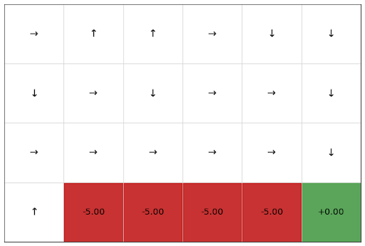
Example: Cliffworld

Q-learning

SARSA

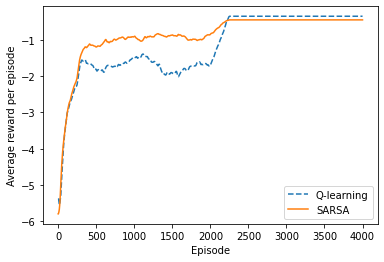
Example: Cliffworld

Question: How do we choose between using on- or off-policy methods?

\(n\)-step TD

Let TD target look \(n\) steps into the future

n-Step Return

Consider the following \(n\)-step returns for \(n=1, 2, \infty\): \[\begin{align*} \color{red}{n} & \color{red}{= 1}\ \text{(TD(0))} & G_t^{(1)} & = r_{t+1} + \gamma V(s_{t+1})\\[2pt] \color{red}{n} & \color{red}{= 2} & G_t^{(2)} & = r_{t+1} + \gamma r_{t+2} + \gamma^2 V(s_{t+2})\\[2pt] \color{red}{\vdots} & & \vdots & \\[2pt] \color{red}{n} & \color{red}{= \infty}\ \text{(MC)} & G_t^{(\infty)} & = r_{t+1} + \gamma r_{t+2} + \cdots + \gamma^{T-1} r_T \end{align*}\]

Define the \(n\)-step Return (real reward \(+\) estimated reward, \({\color{blue}{\gamma^n V(s_{t+n})}}\)):

\[ G^{(n)}_t = r_{t+1} + \gamma r_{t+2} + \cdots + \gamma^{n-1} r_{t+n} + {\color{blue}{\gamma^n V(s_{t+n})}} \]

\(n\)-step temporal-difference learning (updated in direction of error)

\[ Q(s_t, a_t) \;\leftarrow\; Q(s_t, a_t) + \alpha \big({\color{red}{G_t^{(n)} - Q(s_t, a_t)}} \big) \]

\(\lambda\)-return

The \(\lambda\)-return \(G_t^{\lambda}\) combines all \(n\)-step returns \(G_t^{(n)}\)

Using weight \({\color{red}{(1 - \lambda)\lambda^{\,n-1}}}\)

\[ G_t^{\lambda} \;=\; {\color{red}{(1 - \lambda) \sum_{n=1}^{\infty} \lambda^{\,n-1}}} G_t^{(n)} \]

Forward-view TD(\(\lambda\))

\[ Q(s_t, a_t) \;\leftarrow\; Q(s_t, a_t) + \alpha \big( G_t^{\lambda} - Q(s_t, a_t) \big) \]

TD(\(\lambda\)) Weighting Function

\[ G_t^{\lambda} \;=\; (1 - \lambda) \sum_{n=1}^{\infty} \lambda^{\,n-1} G_t^{(n)} \]

\(\lambda\)-return is a geometrically weighted return for every \(n\)-step return

Forward View of TD(λ)

Update value function towards the \(\lambda\)-return

Forward-view looks into the future to compute \(G^{\lambda}_t\)
Like MC, can only be computed from complete episodes

Backward View of TD(\(\lambda\))

Forward view provides theory
Backward view provides mechanism
Update online, every step, from incomplete sequences

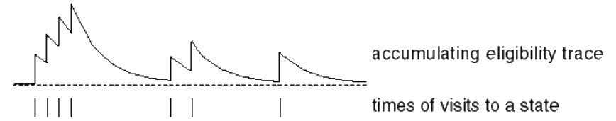
Eligibility Traces

Credit assignment problem: did bell or light cause shock?

Frequency heuristic: assign credit to most frequent states
Recency heuristic: assign credit to most recent states
Eligibility traces combine both heuristics

\[\begin{align*} E_0(s, a) & = 0\\[2pt] E_t(s, a) & = \gamma \lambda E_{t-1}(s) + 1(\text{iff } (s_t, a_t) = (s, a)) \end{align*}\]

Backward View TD(\(\lambda\))

Keep an eligibility trace for every state-action pair \(E(s, a)\)
For every pair \((s, a)\), update \(Q(s, a)\) in proportion to TD-error \(\delta_t\) and eligibility trace \(E_t(s, a)\)

\[ \delta_t = (r_{t+1} + \gamma V(s_{t+1})) - Q(s_t, a_t) \]

\[ Q(s, a) \;\leftarrow\; Q(s, a) + \alpha \,\delta_t E_t(s, a) \]

TD(\(\lambda\)) and TD(\(0\))

When \(\lambda = 0\), only the current state-action pair is updated.

\[E_t(s, a) = \mathbf{1}(\text{iff } s_t = s, a_t = a)\] \[Q(s, a) \leftarrow Q(s, a) + \alpha\,\delta_t\,E_t(s, a)\]

This is exactly equivalent to the TD(\(0\)) update.

\[Q(s_t, a_t) \leftarrow Q(s_t, a_t) + \alpha\,\delta_t\]

TD(\(\lambda\)) and MC

When \(\lambda = 1\), credit is deferred until the end of the episode.

Consider episodic environments with offline updates.
Over the course of an episode, the total update for TD(\(\lambda\)) is the same as the total update for MC.

Theorem

The sum of offline updates is identical for forward-view and backward-view TD(\(\lambda\)):

\[ \sum_{t=1}^{T} \alpha\,\delta_t\,E_t(s, a) \;=\; \sum_{t=1}^{T} \alpha \bigl( G_t^{\lambda} - Q(s_t, a_t) \bigr)\,\mathbf{1}(s_t = s, a_t = a). \]