Appendix (Additional Examples & Reference Material)

Table of contents

• Appendix (Additional Examples & Reference Material)
• Markov Decision Processes (MDPs) - Additional Examples
• Optimal Value Function
• Model-Based Reinforcement Learning
• Model-Based and Model-Free RL
• Learning a Model
• Computational Complexity of Planning
• Convergence & Contraction Mapping Theorem
• Relationship Between Forward and Backward TD
• Linear Least Squares Methods
• Natural Actor-Critic (Advanced Topic)

Appendix (Additional Examples & Reference Material)

Markov Decision Processes (MDPs) - Additional Examples

Markov decision processes formally describe an environment for reinforcement learning

Where the environment is fully observable -i.e. The current state completely characterises the process

Almost all RL problems can be formalised as MDPs, e.g.

• Optimal control primarily deals with continuous MDPs
• Partially observable problems can be converted into MDPs
• Bandits (from machine learning) are MDPs with just one state

Markov Decision Process

A Markov decision process (MDP) is a Markov reward process with decisions.

• It is an environment in which all states are Markov.

• We introduced agency in terms of actions.

Definition

A Markov Decision Process is a tuple \(<\mathcal{S}, \mathcal{\textcolor{red}{A}}, \mathcal{P}, \mathcal{R}, \gamma>\)

• \(\mathcal{S}\) is a finite set of states

• \(\mathcal{\color{red}{A}}\) is a finite set of actions

• \(\mathcal{P}\) is a state transition probability matrix, \(P^{\textcolor{red}{a}}_{ss'} = \mathbb{P} [S_{t+1} = s'\ | S_t = s, A_t = \textcolor{red}{a}]\)

• \(\mathcal{R}\) is a reward function, \(\mathcal{R}^{\textcolor{red}{a}}_s = \mathbb{E}[R_{t+1}\ |\ S_t = s, A_t = {\textcolor{red}{a}}]\)

• \(\gamma\) is a discount factor \(\gamma \in [0,1]\).

Example: Student MDP

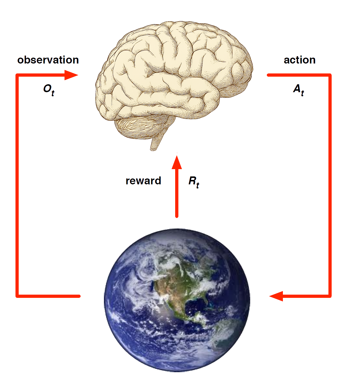
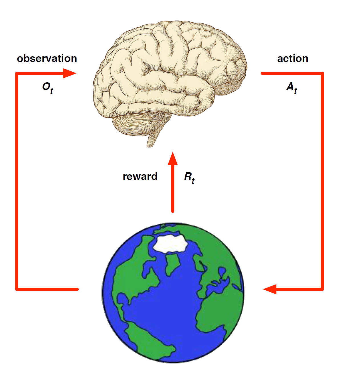
Agent exerts control over MDP via actions, and goal is to find the best path through decision making process to maximise rewards

Policies (1)

Definition

A (stochastic) policy \(\pi\) is a distribution over actions given states,

\[ \pi(a \mid s) = \mathbb{P}\!\left[\, A_t = a \;\middle|\; S_t = s \,\right] \]

• A policy fully defines the behaviour of an agent

• MDP policies depend on the current state (not the history)

• i.e. Policies are stationary (time-independent), \(A_t \sim \pi(\,\cdot \mid S_t), \quad \forall t > 0\)

Policies (2) - Recovering Markov reward process from MDP

Given an MDP \(\mathcal{M} = \langle \mathcal{S}, \mathcal{A}, \mathcal{P}, \mathcal{R}, \gamma \rangle\) and a policy \(\pi\)

• The state sequence \(S_1, S_2, \ldots\) is a Markov process \(\langle \mathcal{S}, \mathcal{P}^\pi \rangle\)

• The state and reward sequence \(S_1, R_2, S_2, \ldots\) is a Markov reward process \(\langle \mathcal{S}, \mathcal{P}^\pi, \mathcal{R}^\pi, \gamma \rangle\), where

\[ \mathcal{P}^{\pi}_{s,s'} = \sum_{a \in \mathcal{A}} \pi(a \mid s)\, \mathcal{P}^{a}_{s s'} \]

\[ \mathcal{R}^{\pi}_{s} = \sum_{a \in \mathcal{A}} \pi(a \mid s)\, \mathcal{R}^{a}_{s} \]

Value Function

Definition

The state-value function \(v_\pi(s)\) of an MDP is the expected return starting from state \(s\), and then following policy \(\pi\)

\[ v_\pi(s) = \mathbb{E}_\pi \!\left[\, G_t \;\middle|\; S_t = s \,\right] \]

Definition

The action-value function \(q_\pi(s, a)\) is the expected return starting from state \(s\), taking action \(a\), and then following policy \(\pi\)

\[ q_\pi(s, a) = \mathbb{E}_\pi \!\left[\, G_t \;\middle|\; S_t = s,\, A_t = a \,\right] \]

Example: State-Value Function for Student MDP

Bellman Expectation Equation

The state-value function can again be decomposed into immediate reward plus discounted value of successor state,

\[ v_\pi(s) = \mathbb{E}_\pi \!\left[\, R_{t+1} + \gamma v_\pi(S_{t+1}) \;\middle|\; S_t = s \,\right] \]

Can do the same thing for the \(q\) values: the action-value function can similarly be decomposed,

\[ q_\pi(s, a) = \mathbb{E}_\pi \!\left[\, R_{t+1} + \gamma q_\pi(S_{t+1}, A_{t+1}) \;\middle|\; S_t = s,\, A_t = a \,\right] \]

Bellman Expectation Equation for \(V^{\pi}\) (look ahead)

 

\[ v_\pi(s) = \sum_{a \in \mathcal{A}} \pi(a \mid s)\, q_\pi(s, a) \]

Bellman Expectation Equation for \(Q^{\pi}\) (look ahead)

 

\[ q_\pi(s, a) = \mathcal{R}^a_s + \gamma \sum_{s' \in \mathcal{S}} \mathcal{P}^a_{s s'}\, v_\pi(s') \]

Bellman Expectation Equation for \(v_{\pi} (2)\)

Bringing it together: agent actions (open circles), environment actions (closed circles)

\[ v_\pi(s) = \sum_{a \in \mathcal{A}} \pi(a \mid s) \left( \mathcal{R}^a_s + \gamma \sum_{s' \in \mathcal{S}} \mathcal{P}^a_{s s'} \, v_\pi(s') \right) \]

Bellman Expectation Equation for \(q_{\pi} (2)\)

The other way around: can do same thing for action values

\[ q_\pi(s, a) = \mathcal{R}^a_s + \gamma \sum_{s' \in \mathcal{S}} \mathcal{P}^a_{s s'} \sum_{a' \in \mathcal{A}} \pi(a' \mid s') \, q_\pi(s', a') \]

In both forms value function is (recursively) equal to reward of immediate state \(s\) + value \(s'\) (where you end up)

Example: Bellman Expectation Equation in Student MDP

Verify Bellman Equation to compute \(v_{\pi}(s)\) for \(s=C3\)

Bellman Expectation Equation (Matrix Form)

The Bellman expectation equation can be expressed concisely using the induced MRP (as before),

\[ v_\pi = \mathcal{R}^\pi + \gamma \mathcal{P}^\pi v_\pi \]

with direct solution

\[ v_\pi = (I - \gamma \mathcal{P}^\pi)^{-1} \mathcal{R}^\pi \]

• Bellman equation gives us description of system can solve

• Essentially averaging then computing inverse, although inefficient!

Optimal Value Function

Optimal Value Function (Finding the best behaviour)

Definition

The optimal state-value function \(v_\ast(s)\) is the maximum value function over all policies

\[ v_\ast(s) = \max_{\pi} v_\pi(s) \]

The optimal action-value function \(q_\ast(s, a)\) is the maximum action-value function over all policies

\[ q_\ast(s, a) = \max_{\pi} q_\pi(s, a) \]

• The optimal value function specifies the best possible performance in the MDP.

• An MDP is “solved” when we know the optimal value function.

• If you know \(q_\ast\), you have the optimal value function

• So solving means finding \(q_\ast\)

Example: Optimal Value Function for Student MDP

Gives us value function for each state \(s\) (not how to behave)

Example: Optimal Action-Value Function for Student MDP

Gives us best action, \(a\), for each state \(s\) (can choose)

Optimal Policy

Define a partial ordering over policies

\[ \pi \;\geq\; \pi' \quad \text{if } v_\pi(s) \;\geq\; v_{\pi'}(s), \;\forall s \]

Theorem For any Markov Decision Process

• There exists an optimal policy \(\pi_\ast\) that is better than or equal to all other policies, \(\pi_\ast \geq \pi, \;\forall \pi\)

• All optimal policies achieve the optimal value function, \(v_{\pi_\ast}(s) = v_\ast(s)\)

• All optimal policies achieve the optimal action-value function, \(q_{\pi_\ast}(s,a) = q_\ast(s,a)\)

Finding an Optimal Policy

An optimal policy can be found by maximising over \(q_\ast(s,a)\),

\[ \pi_\ast(a \mid s) = \begin{cases} 1 & \text{if } a = \underset{a \in \mathcal{A}}{\arg\max}\; q_\ast(s,a) \\[6pt] 0 & \text{otherwise} \end{cases} \]

• There is always a deterministic optimal policy for any MDP
• If we know \(q_\ast(s,a)\), we immediately have the optimal policy

Example: Optimal Policy for Student MDP

Red arcs (actions) represent optimal policy: picks highest \(q_\ast\)

Bellman Optimality Equation for \(v_\ast\) (look ahead)

The optimal value functions are recursively related by the Bellman optimality equations:

\[ v_\ast(s) = \max\limits_{a} q_\ast(s,a) \]

Working backwards using backup diagrams we get \(v_\ast(s)\) - best action over all policies taking max instead of average

Bellman Optimality Equation for \(Q^\ast\) (look ahead)

 

\[ q_\ast(s,a) = \mathcal{R}^a_s + \gamma \sum_{s' \in \mathcal{S}} \mathcal{P}^a_{ss'} \, v_\ast(s') \]

Considers where the environment might take us by averaging (looking ahead) and backing up (inductively)

Bellman Optimality Equation for \(V^* (2)\)

Bringing it together (two-step look ahead): agent actions (open circles), environment actions (closed circles)

\[ v_\ast(s) = \max\limits_{a} \mathcal{R}^a_s + \gamma \sum_{s' \in \mathcal{S}} \mathcal{P}^a_{ss'} \, v_\ast(s') \]

Bellman Optimality Equation for \(Q^* (2)\)

 

\[ q_\ast(s,a) = \mathcal{R}^a_s + \gamma \sum_{s' \in \mathcal{S}} \mathcal{P}^a_{ss'} \, \max\limits_{a'} q_\ast(s',a') \]

Determines \(Q^{\ast}\) reordering from environments perspective

Example: Bellman Optimality Equation in Student MDP

Compute \(v_{\ast}(s)\) for \(s=C1\) looking one step ahead (no environment actions in \(C1\))

Solving the Bellman Optimality Equation

Bellman Optimality Equation is non-linear

• No closed form solution (in general)

Many iterative solution methods

• Value Iteration (not covered in this subject)
• Policy Iteration (not covered in this subject)
• Q-learning (covered in Module 9)
• SARSA (covered in Module 9)

Model-Based Reinforcement Learning

Last Module: Learning & Relxation

This Module: learn model directly from experience

• \(\ldots\) and use planning to construct a value function or policy

Integrates learning and planning into a single architecture

Model-Based Reinforcement Learning

Model-Based and Model-Free RL

Model-Free RL

• No model

• Learn value function (and/or policy) from experience

Model-Based RL

• Learn a model from experience

• Plan value function (and/or policy) from model

Lookahead by planning (or thinking) about what the value function will be

Model-Free RL

Model-Based RL

Replace real world with the agent’s (simulated) model of the environment

• Supports rollouts (lookaheads) under imagined actions to reason about what value function will be, without further environment interaction

Model-Based RL (2)

Advantages of Model-Based RL

Advantages:

• Can efficiently learn model by supervised learning methods

• Can reason about model uncertainty, and even take actions to reduce uncertainty

Disadvantages:

• First learn a model, then construct a value function

\(\;\;\;\Rightarrow\) two sources of approximation error

Learning a Model

What is a Model?

A model \(\mathcal{M}\) is a representation of an MDP \(\langle \mathcal{S}, \mathcal{A}, \mathcal{P}, \mathcal{R} \rangle\), parameterised by \(\eta\)

• We will assume state space \(\mathcal{S}\) and action space \(\mathcal{A}\) are known

So a model \(\mathcal{M} = \langle \mathcal{P}_\eta, \mathcal{R}_\eta \rangle\) represents state transitions
\(\mathcal{P}_\eta \approx \mathcal{P}\) and rewards \(\mathcal{R}_\eta \approx \mathcal{R}\)

\[ S_{t+1} \sim \mathcal{P}_\eta(S_{t+1} \mid S_t, A_t) \]

\[ R_{t+1} = \mathcal{R}_\eta(R_{t+1} \mid S_t, A_t) \]

Typically assume conditional independence between state transitions and rewards

\[ \mathbb{P}[S_{t+1}, R_{t+1} \mid S_t, A_t] \;=\; \mathbb{P}[S_{t+1} \mid S_t, A_t] \; \mathbb{P}[R_{t+1} \mid S_t, A_t] \]

Note you can learn from each (one-step) transition, treating the following step as the supervisor for the prior step.

Model Learning

Goal: estimate model \(\mathcal{M}_\eta\) from experience \(\{S_1, A_1, R_2, \ldots, S_T\}\)

This is a supervised learning problem

\[ \begin{aligned} S_1, A_1 &\;\to\; R_2, S_2 \\ S_2, A_2 &\;\to\; R_3, S_3 \\ &\;\vdots \\ S_{T-1}, A_{T-1} &\;\to\; R_T, S_T \end{aligned} \]

• Learning \(s,a \to r\) is a regression problem

• Learning \(s,a \to s'\) is a density estimation problem

• Pick loss function, e.g. mean-squared error, KL divergence, …

• Find parameters \(\eta\) that minimise empirical loss

Examples of Models

• Table Lookup Model

• Linear Expectation Model

• Linear Gaussian Model

• Gaussian Process Model

• Deep Belief Network Model

• \(\cdots\) almost any supervised learning model

Table Lookup Model

Model is an explicit MDP, \(\hat{\mathcal{P}}, \hat{\mathcal{R}}\)

• Count visits \(N(s,a)\) to each state–action pair (parametric approach)

\[ \begin{align*} \hat{\mathcal{P}}^{a}_{s,s'} & = \frac{1}{N(s,a)} \sum_{t=1}^T \mathbf{1}(S_t, A_t, S_{t+1} = s, a, s')\\[0pt] \hat{\mathcal{R}}^{a}_{s} & = \frac{1}{N(s,a)} \sum_{t=1}^T \mathbf{1}(S_t, A_t = s, a)\, R_t \end{align*} \]

• Alternatively (a simple non-parametric approach)
  • At each time-step \(t\), record experience tuple \(\langle S_t, A_t, R_{t+1}, S_{t+1} \rangle\)
  • To sample model, randomly pick tuple matching \(\langle s,a,\cdot,\cdot \rangle\)

AB Example (Revisited) - Building a Model

Two states \(A,B\); no discounting; \(8\) episodes of experience

\(A, 0, B, 0\)

\(B, 1\)

\(B, 1\)

\(B, 1\)

\(B, 1\)

\(B, 1\)

\(B, 1\)

\(B, 0\)

We have constructed a table lookup model from the experience

Computational Complexity of Planning

Algorithmic Problems in Planning

Satisficing Planning

Input: A planning task \(P\).
Output: A plan for \(P\), or unsolvable if no plan for \(P\) exists.

Optimal Planning

Input: A planning task \(P\).
Output: An optimal plan for \(P\), or unsolvable if no plan for \(P\) exists.

\(\rightarrow\) The techniques successful for either one of these are almost disjoint!

\(\rightarrow\) Satisficing planning is much more effective in practice

\(\rightarrow\) Programs solving these problems are called planners, planning systems, or planning tools.

Decision Problems in Planning

Definition (PlanEx). By PlanEx, we denote the problem of deciding, given a planning task \(P\), whether or not there exists a plan for \(P\).

\(\rightarrow\) Corresponds to satisficing planning.

 

Definition (PlanLen). By PlanLen, we denote the problem of deciding, given a planning task \(P\) and an integer \(B\), whether or not there exists a plan for \(P\) of length at most \(B\).

\(\rightarrow\) Corresponds to optimal planning.

NP & PSPACE Classes (Refresher)

NP: Decision problems for which there exists a non-deterministic Turing machine that runs in time polynomial in the size of its input.

• Accepts if at least one of the possible runs accepts.

PSPACE: Decision problems for which there exists a deterministic Turing machine that runs in space polynomial in the size of its input.

 

Relationship between classes: Non-deterministic polynomial space can be simulated in deterministic polynomial space.

• Thus PSPACE = NPSPACE, and hence (trivially) NP \(\subset\) PSPACE.

For details see a computational complexity textbook, such as Garey and Johnson (1979).

Computational Complexity of PlanEx and PlanLen

Theorem. PlanEx and PlanLen are PSPACE-complete.

• “At least as hard as any other problem contained in PSPACE.”
• Details: Bylander (1994).

Domain-Specific PlanEx vs. PlanLen

• In general, both have the same complexity.
• Within particular applications, bounded length plan existence is often harder than plan existence.
• This happens in many IPC benchmark domains: PlanLen is NP-complete while PlanEx is in P.
  • For example: Blocksworld and Logistics.
• In practice, optimal planning is (almost) never “easy”.

Is Blocksworld Hard?

Blocksworld is Hard!

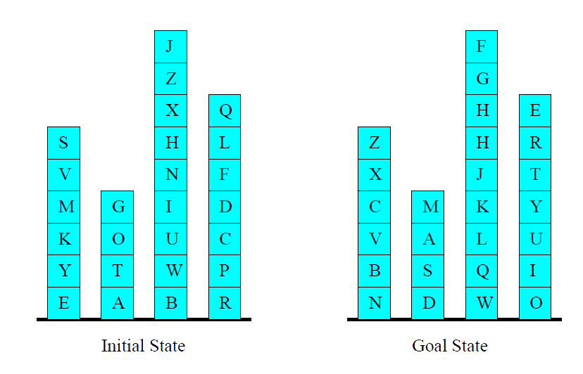
Why All the Fuss? Example Blocksworld

• \(n\) blocks, \(1\) hand.
• A single action either takes a block with the hand or puts a block we’re holding onto some other block/the table.

State Space Growth in Blocksworld

blocks	states
1	1
2	3
3	13
4	73
5	501
6	4051
7	37633
8	394353 …

blocks	states
9	4596553
10	58941091
11	824073141
12	12470162233
13	202976401213
14	3535017524403
15	65573803186921
16	1290434218669921

\(\rightarrow\) State spaces may be huge. In particular, the state space is typically exponentially large in the size of its specification via the problem \(\Pi\) (up next).

\(\rightarrow\) In other words: search problems typically are computationally hard (e.g., optimal Blocksworld solving is NP-complete).

Convergence & Contraction Mapping Theorem

Convergence?

How do we know that value iteration converges to \(v_*\)?

Or that iterative policy evaluation converges to \(v_{\pi}\)?

And therefore that policy iteration converges to \(v_*\)?

Is the solution unique?

How fast do these algorithms converge?

These questions are resolved by contraction mapping theorem

Value Function Space

Consider the vector space \(\mathcal{V}\) over value functions

• There are \(|\mathcal{S}|\) dimensions

• Each point in this space fully specifies a value function \(v(s)\)

What does a Bellman backup do to points in this space?

• We will show that it brings value functions closer,

• \(\ldots\) and therefore the backups must converge on a unique solution

Value Function \(\infty\)-Norm

We will measure distance between state-value functions \(u\) and \(v\) by the \(\infty\)-norm

i.e. the largest difference between state values,

\[ \|u - v\|_{\infty} = \max_{s \in \mathcal{S}} |u(s) - v(s)| \]

Bellman Expectation Backup is a Contraction

Define the Bellman expectation backup operator \(T^{\pi}\)

\[ T^{\pi}(v) = \mathcal{R}^{\pi} + \gamma \mathcal{P}^{\pi} v \]

This operator is a \(\gamma\)-contraction, i.e. it makes value functions closer by at least \(\gamma\):

\[ \begin{align*} \|T^{\pi}(u) - T^{\pi}(v)\|_{\infty} &= \|(\mathcal{R}^{\pi} + \gamma \mathcal{P}^{\pi} u) - (\mathcal{R}^{\pi} + \gamma \mathcal{P}^{\pi} v)\|_{\infty} \\[4pt] &= \|\gamma \mathcal{P}^{\pi} (u - v)\|_{\infty} \\[4pt] &\le \|\gamma \mathcal{P}^{\pi}\|_{\infty} \, \|u - v\|_{\infty} \\[4pt] &\le \gamma \, \|u - v\|_{\infty} \end{align*} \]

Contraction Mapping Theorem

Theorem (Contraction Mapping Theorem)

For any metric space \(\mathcal{V}\) that is complete (i.e. closed) under an operator \(T(v)\), where \(T\) is a \(\gamma\)-contraction,

• \(T\) converges to a unique fixed point

• At a linear convergence rate of \(\gamma\)

Convergence of Policy Evaluation and Policy Iteration

The Bellman expectation operator \(T^{\pi}\) has a unique fixed point

\(v_{\pi}\) is a fixed point of \(T^{\pi}\) (by the Bellman expectation equation)

By the contraction mapping theorem

Iterative policy evaluation converges on \(v_{\pi}\)

Policy iteration converges on \(v_{*}\)

Bellman Optimality Backup is a Contraction

Define the Bellman optimality backup operator \(T^{*}\),

\[ T^{*}(v) = \max_{a \in \mathcal{A}} \left( \mathcal{R}^{a} + \gamma \mathcal{P}^{a} v \right) \]

This operator is a \(\gamma\)-contraction,
i.e. it makes value functions closer by at least \(\gamma\)
(similar to previous proof)

\[ \|T^{*}(u) - T^{*}(v)\|_{\infty} \le \gamma \|u - v\|_{\infty} \]

Convergence of Value Iteration

The Bellman optimality operator \(T^*\) has a unique fixed point

\(v_*\) is a fixed point of \(T^*\) (by Bellman optimality equation)

By contraction mapping theorem

Value iteration converges on \(v_*\)

Relationship Between Forward and Backward TD

TD(\(\lambda\)) and TD(\(0\))

When \(\lambda = 0\), only the current state is updated

\[ \begin{align*} E_t(s) & = \mathbf{1}(S_t = s)\\[0pt] V(s) & \leftarrow V(s) + \alpha \delta_t E_t(s) \end{align*} \]

This is exactly equivalent to the TD(\(0\)) update

\[ V(S_t) \leftarrow V(S_t) + \alpha \delta_t \]

TD(\(\lambda\)) and MC(\(0\))

When \(\lambda = 1\), credit is deferred until the end of the episode

• Consider episodic environments with offline updates

• Over the course of an episode, total update for TD(\(1\)) is the same as total update for MC

Theorem

The sum of offline updates is identical for forward-view and backward-view TD(\(\lambda\))

\[ \sum_{t=1}^{T} \alpha \delta_t E_t(s) = \sum_{t=1}^{T} \alpha \left( G_t^{\lambda} - V(S_t) \right) \mathbf{1}(S_t = s) \]

MC and TD(\(1\))

Consider an episode where \(s\) is visited once at time-step \(k\)

• TD(1) eligibility trace discounts time since visit:

\[ \begin{align*} E_t(s) & = \gamma E_{t-1}(s) + \mathbf{1}(S_t = s)\\[0pt] & = \begin{cases} 0, & \text{if } t < k \\ \gamma^{t-k}, & \text{if } t \ge k \end{cases} \end{align*} \]

• TD(1) updates accumulate error online:

\[ \sum_{t=1}^{T-1} \alpha \delta_t E_t(s) = \alpha \sum_{t=k}^{T-1} \gamma^{t-k} \delta_t = \alpha (G_k - V(S_k)) \]

• By the end of the episode, it accumulates total error:

\[ \delta_k + \gamma \delta_{k+1} + \gamma^2 \delta_{k+2} + \dots + \gamma^{T-1-k} \delta_{T-1} \]

Telescoping in TD(\(1\))

When \(\lambda = 1\), the sum of TD errors telescopes into the Monte Carlo (MC) error:

\[ \begin{align*} & \delta_t + \gamma \delta_{t+1} + \gamma^{2}\delta_{t+2} + \dots + \gamma^{T-1-t}\delta_{T-1}\\[0pt] & =\; R_{t+1} + \gamma V(S_{t+1}) - V(S_t)\\[0pt] & +\; \gamma R_{t+2} + \gamma^{2} V(S_{t+2}) - \gamma V(S_{t+1})\\[0pt] & +\; \gamma^{2} R_{t+3} + \gamma^{3} V(S_{t+3}) - \gamma^{2} V(S_{t+2})\\[0pt] & \quad \quad \quad \vdots\\[0pt] & +\; \gamma^{T-1-t} R_T + \gamma^{T-t} V(S_T) - \gamma^{T-1-t} V(S_{T-1})\\[0pt] & =\; R_{t+1} + \gamma R_{t+2} + \gamma^{2} R_{t+3} + \dots + \gamma^{T-1-t} R_T - V(S_t)\\[0pt] & =\; G_t - V(S_t) \end{align*} \]

TD(\(\lambda\)) and TD(\(1\))

TD(\(1\)) is roughly equivalent to every-visit Monte-Carlo

Error is accumulated online, step-by-step

If value function is only updated online at end of episode

Then total update is exactly the same as MC

Telescoping in TD(\(\lambda\))

For general \(\lambda\), TD errors also telescope to the \(\lambda\)-error, \(G_t^{\lambda} - V(S_t)\)

\[ \begin{align*} & G_t^{\lambda}-V(S_t)\hspace{-15mm} &=-V(S_t) &+(1-\lambda)\lambda^{0}(R_{t+1} + \gamma V(S_{t+1}))\\[0pt] & & &+(1-\lambda)\lambda^{1}(R_{t+1}+\gamma R_{t+2}+\gamma^{2} V(S_{t+2})) \\[0pt] & & & + (1 - \lambda)\lambda^{2}(R_{t+1} + \gamma R_{t+2} + \gamma^{2} R_{t+3} + \gamma^{3} V(S_{t+3}))\\[0pt] & & &+ \dots \\[0pt] & &= -V(S_t) &+(\gamma\lambda)^{0}(R_{t+1}+\gamma V(S_{t+1})-\gamma\lambda V(S_{t+1})) \\[0pt] & & & + (\gamma\lambda)^{1}(R_{t+2} + \gamma V(S_{t+2}) - \gamma\lambda V(S_{t+2})) \\[0pt] & & & + (\gamma\lambda)^{2}(R_{t+3} + \gamma V(S_{t+3}) - \gamma\lambda V(S_{t+3})) \\[0pt] & & & + \dots \\[0pt] & &= \quad \quad \quad \quad & \quad (\gamma\lambda)^{0}(R_{t+1} + \gamma V(S_{t+1}) - V(S_t)) \\[0pt] & & & + (\gamma\lambda)^{1}(R_{t+2} + \gamma V(S_{t+2}) - V(S_{t+1})) \\[0pt] & & & + (\gamma\lambda)^{2}(R_{t+3} + \gamma V(S_{t+3}) - V(S_{t+2})) \\[0pt] & & & + \dots \\[0pt] & & & \hspace{-37mm} = \delta_t + \gamma\lambda \delta_{t+1} + (\gamma\lambda)^2 \delta_{t+2} + \dots \end{align*} \]

Forwards and Backwards TD(\(\lambda\))

Consider an episode where \(s\) is visited once at time-step \(k\)

TD(\(\lambda\)) eligibility trace discounts time since visit:

\[ \begin{align*} E_t(s) & = \gamma \lambda E_{t-1}(s) + \mathbf{1}(S_t = s)\\[0pt] & = \begin{cases} 0, & \text{if } t < k \\ (\gamma \lambda)^{t-k}, & \text{if } t \ge k \end{cases} \end{align*} \]

Backward TD(\(\lambda\)) updates accumulate error online:

\[ \sum_{t=1}^{T} \alpha \delta_t E_t(s) = \alpha \sum_{t=k}^{T} (\gamma \lambda)^{t-k} \delta_t = \alpha \left(G_k^{\lambda} - V(S_k)\right) \]

• By the end of the episode, it accumulates total error for the \(\lambda\)-return

• For multiple visits to \(s\), \(E_t(s)\) accumulates many errors

Offline Equivalence of Forward and Backward TD

Offline updates

• Updates are accumulated within episode

• but applied in batch at the end of episode

Online Equivalence of Forward and Backward TD

Online updates

• TD(\(\lambda\)) updates are applied online at each step within episode

• Forward and backward-view TD(\(\lambda\)) are slightly different

• Exact online TD(\(\lambda\)) achieves perfect equivalence

• By using a slightly different form of eligibility trace

Harm van Seijen, A. Rupam Mahmood, Patrick M. Pilarski, Marlos C. Machado, Richard S. Sutton; True Online Temporal-Difference Learning. Journal of Machine Learning Research (JMLR), 17(145):1−40, 2016.

Summary of Forward and Backward TD(\(\lambda\))

\[ \begin{array}{|c|c|c|c|} \hline {\color{red}{\text{Offline updates}}} & {\color{red}{\lambda = 0}} & {\color{red}{\lambda \in (0,1)}} & {\color{red}{\lambda = 1}} \\ \hline \text{Backward view} & \text{TD(0)} & \text{TD}(\lambda) & \text{TD(1)} \\[0pt] & || & || & || \\[0pt] \text{Forward view} & \text{TD(0)} & \text{Forward TD}(\lambda) & \text{MC} \\[0pt] \hline {\color{red}{\text{Online updates}}} & {\color{red}{\lambda = 0}} & {\color{red}{\lambda \in (0,1)}} & {\color{red}{\lambda = 1}} \\ \hline \text{Backward view} & \text{TD(0)} & \text{TD}(\lambda) & \text{TD(1)} \\[0pt] & || & \neq & \neq \\[0pt] \text{Forward view} & \text{TD(0)} & \text{Forward TD}(\lambda) & \text{MC} \\[0pt] & || & || & || \\[0pt] \text{Exact Online} & \text{TD(0)} & \text{Exact Online TD}(\lambda) & \text{Exact Online TD(1)} \\ \hline \end{array} \]

= here indicates equivalence in total update at end of episode.

Linear Least Squares Methods

Linear Least Squares Prediction

Experience replay finds the least squares solution

• But may take many iterations.

Using the special case of linear value function approximation

\[ \hat{v}(s,\mathbf{w}) = x(s)^\top \mathbf{w} \]

We can solve the least squares solution directly using a closed form

Linear Least Squares Prediction (2)

At the minimum of \(LS(\mathbf{w})\), the expected update must be zero:

\[\begin{align*} \mathbb{E}_{\mathcal{D}} \left[ \Delta \mathbf{w} \right] &= 0\;\;\; \text{(want update zero across data set)} \\[0pt] \alpha \sum_{t=1}^{T} \mathbf{x}(s_t) \bigl( v_t^{\pi} - \mathbf{x}(s_t)^{\top} \mathbf{w} \bigr) &= 0\;\;\; \text{(unwrapping expected updates)}\\[0pt] \sum_{t=1}^{T} \mathbf{x}(s_t) v_t^{\pi} &= \sum_{t=1}^{T} \mathbf{x}(s_t) \mathbf{x}(s_t)^{\top} \mathbf{w} \\[0pt] \mathbf{w} &= \left( \sum_{t=1}^{T} \mathbf{x}(s_t) \mathbf{x}(s_t)^{\top} \right)^{-1} \sum_{t=1}^{T} \mathbf{x}(s_t) v_t^{\pi} \end{align*}\]

Compute time: \(O(N^3)\) for \(N\) features (direct),
or incremental \(O(N^2)\) using Sherman–Morrison.

• Sometimes better or cheaper than experience replay, e.g. if have only a few features for the linear cases.

Linear Least Squares Prediction Algorithms

We do not know true values \(v_t^\pi\)

• In practice, our “training data” must use noisy or biased samples of \(v^{\pi}_t\)

\[\begin{align*} {\color{blue}{\text{LSMC}}} \;\;\;\;&\text{Least Squares Monte-Carlo uses return}\\[0pt] & v_t^\pi \approx {\color{red}{G_t}} \\[0pt] {\color{blue}{\text {LSTD}}} \;\;\;\; & \text{Least Squares Temporal-Difference uses TD target}\\[0pt] & v_t^\pi \approx {\color{red}{R_{t+1} + \gamma \hat{v}(S_{t+1}, \mathbf{w})}}\\[0pt] {\color{blue}{\text{LSTD}}}{\color{blue}{(\lambda)}}\;\;\;\; & \text{Least Squares TD}(\lambda)\text{ uses}\;\lambda\text{-return} \\[0pt] & v_t^\pi \approx {\color{red}{G_t^\lambda}} \end{align*}\]

In each case we can solve directly for the fixed point of MC / TD / TD(\(\lambda\))

Linear Least Squares Prediction Algorithms (2)

\[\begin{align*} {\color{red}{\text{LSMC}}} \;\;\;\; 0 & = \sum_{t=1}^T \alpha \big(G_t - \hat{v}(S_t,\mathbf{w})\big)\, \textbf{x}(S_t),\qquad\\[0pt] \mathbf{w} & = \left(\sum_{t=1}^T \textbf{x}(S_t) \textbf{x}(S_t)^\top \right)^{-1} \left(\sum_{t=1}^T \textbf{x}(S_t) G_t \right)\\[0pt] {\color{red}{\text{LSTD}}} \;\;\;\; 0 & = \sum_{t=1}^T \alpha \big(R_{t+1} + \gamma \hat{v}(S_{t+1},\mathbf{w}) - \hat{v}(S_t,\mathbf{w})\big)\, \textbf{x}(S_t)\\[0pt] \mathbf{w} & = \left(\sum_{t=1}^T \textbf{x}(S_t)\big(x(S_t) - \gamma \textbf{x}(S_{t+1})\big)^\top \right)^{-1} \left(\sum_{t=1}^T \textbf{x}(S_t) R_{t+1}\right)\\[0pt] {\color{red}{\text{LSTD}}}{\color{red}{(\lambda)}}\;\;\;\; 0 & = \sum_{t=1}^T \alpha\, \delta_t\, E_t,\qquad\\[0pt] \mathbf{w} & = \left(\sum_{t=1}^T E_t \big(\textbf{x}(S_t) - \gamma \textbf{x}(S_{t+1})\big)^\top \right)^{-1} \left(\sum_{t=1}^T E_t R_{t+1}\right) \end{align*}\]

Convergence of Linear Least Squares Prediction Algorithms

\[ \begin{array}{l l c c c} \hline \text{On/Off-Policy} & \text{Algorithm} & \text{Table Lookup} & \text{Linear} & \text{Non-Linear} \\ \hline \text{On-Policy} & \textit{MC} & \checkmark & \checkmark & \checkmark \\ & {\color{red}{\textit{LSMC}}} & {\color{red}{\checkmark}} & {\color{red}{\checkmark}} & {\color{red}{-}} \\ & \textit{TD} & \checkmark & \checkmark & \text{✗} \\ & {\color{red}{\textit{LSTD}}} & {\color{red}{\checkmark}} & {\color{red}{\checkmark}} & {\color{red}{-}} \\ \hline \text{Off-Policy} & \textit{MC} & \checkmark & \checkmark & \checkmark \\ & {\color{red}{\textit{LSMC}}} & {\color{red}{\checkmark}} & {\color{red}{\checkmark}} & {\color{red}{-}} \\ & \textit{TD} & \checkmark & \text{✗} & \text{✗} \\ & {\color{red}{\textit{LSTD}}} & {\color{red}{\checkmark}} & {\color{red}{\checkmark}} & {\color{red}{-}} \\ \hline \end{array} \]

Least Squares Policy Iteration

Policy evaluation Policy evaluation by least-squares Q-learning

Policy improvement Greedy policy improvement

Least Squares Action-Value Function Approximation

Approximate action-value function \(q_\pi(s, a)\)

• using linear combination of features \(\mathbf{x}(s, a)\)

\[ \hat{q}(s, a, \mathbf{w}) = \mathbf{x}(s, a)^\top \mathbf{w} \;\approx\; q_\pi(s, a) \]

Minimise least squares error between \(\hat{q}(s, a, \mathbf{w})\) and \(q_\pi(s, a)\)

• from experience generated using policy \(\pi\)

• consisting of \(\langle (state, action), value \rangle\) pairs

\[ \mathcal{D} = \Bigl\{ \langle (s_1, a_1), v_1^\pi \rangle,\; \langle (s_2, a_2), v_2^\pi \rangle,\; \ldots,\; \langle (s_T, a_T), v_T^\pi \rangle \Bigr\} \]

Least Squares Control

For policy evaluation, we want to efficiently use all experience

For control, we also want to improve the policy

The experience is generated from many policies

So to evaluate \(q_\pi(S,A)\) we must learn off-policy

We use the same idea as Q-learning:

• Experience from old policy: \((S_t, A_t, R_{t+1}, S_{t+1}) \sim \pi_{\text{old}}\)
  
• Consider alternative successor action \(A^{\prime} = \pi_{\text{new}}(S_{t+1})\)
  
• Update \(\hat{q}(S_t, A_t, \mathbf{w})\) toward
  \[ R_{t+1} + \gamma\, \hat{q}(S_{t+1}, A^{\prime}, \mathbf{w}) \]

Least Squares Q-Learning

Consider the following linear Q-learning update

\[\begin{align*} \delta &= R_{t+1} + \gamma \hat{q}(S_{t+1}, {\color{red}{\pi(S_{t+1})}}, \mathbf{w}) - \hat{q}(S_t, A_t, \mathbf{w}) \\[0.5em] \Delta \mathbf{w} &= \alpha \, \delta \, \mathbf{x}(S_t, A_t) \end{align*}\]

LSTDQ algorithm: solve for total update \(=\) zero

\[\begin{align*} 0 &= \sum_{t=1}^T \alpha \Big( R_{t+1} + \gamma \hat{q}(S_{t+1}, {\color{red}{\pi(S_{t+1})}}, \mathbf{w}) - \hat{q}(S_t, A_t, \mathbf{w}) \Big)\mathbf{x}(S_t, A_t) \\[1em] \mathbf{w} &= \Bigg( \sum_{t=1}^T \mathbf{x}(S_t, A_t)\big(\mathbf{x}(S_t, A_t) - \gamma \mathbf{x}(S_{t+1}, \pi(S_{t+1}))\big)^\top \Bigg)^{-1} \sum_{t=1}^T \mathbf{x}(S_t, A_t) R_{t+1} \end{align*}\]

Least Squares Policy Iteration Algorithm

The following pseudo-code uses LSTDQ for policy evaluation

It repeatedly re-evaluates experience \(\mathcal{D}\) with different policies

Least Squares Policy Iteration Algorithm (LSTFQ variant)

\[ \begin{aligned} &\text{function LSPI-TD}(\mathcal{D}, \pi_0) \\ &\quad \pi^{\prime} \leftarrow \pi_0 \\ &\quad \text{repeat} \\ &\qquad \pi \leftarrow \pi^{\prime} \\ &\qquad Q \leftarrow \text{LSTDQ}(\pi,\mathcal{D}) \\ &\qquad \text{for all } s \in S \text{ do} \\ &\qquad\quad \pi^{\prime}(s) \leftarrow \arg\max_{a \in A} Q(s,a) \\ &\qquad \text{end for} \\ &\quad \text{until } (\pi \approx \pi^{\prime}) \\ &\quad \text{return } \pi \\ &\text{end function} \end{aligned} \]

Convergence of Control Algorithms

\[ \begin{array}{l l c c c} \hline \text{Algorithm} & \text{Table Lookup} & \text{Linear} & \text{Non-Linear} \\ \hline \textit{Monte-Carlo Control} & \checkmark & (\checkmark) & \text{✗} \\ \textit{Sarsa} & \checkmark & (\checkmark) & \text{✗} \\ \textit{Q-Learning} & \checkmark & \text{✗} & \text{✗} \\ \textit{\color{red}{LSPI}} & \checkmark & (\checkmark) & - \\ \hline \end{array} \]

(\(\checkmark\)) = chatters around near-optimal value function.

Chain Walk Example (More complicated random walk)

Consider the 50 state version of this problem (bigger replica of this diagram)

• Reward \(+1\) in states \(10\) and \(41\), \(0\) elsewhere

• Optimal policy: R (\(1-9\)), L (\(10-25\)), R (\(26-41\)), L (\(42, 50\))

• Features: \(10\) evenly spaced Gaussians (\(\sigma = 4\)) for each action

• Experience: \(10,000\) steps from random walk policy

LSPI in Chain Walk: Action-Value Function

Plots show LSPI iterations on a 50-state chain with a radial basis function approximator.

• The colours represent two different actions of going left (blue) or right (red)

• The plots show the true value function (dashed) or approximate value function

• You can see it converges to the optimal policy after only \(7\) iterations.

LSPI in Chain Walk: Policy

Plots of policy improvement over LSPI iterations (using same 50-state chain example).

• Shows convergence of LSPI policy to optimal within a few iterations.
  

Natural Actor-Critic (Advanced Topic)

Alternative Policy Gradient Directions

Gradient ascent algorithms can follow any ascent direction

• A good ascent direction can significantly speed convergence

Also, a policy can often be reparametrised without changing action probabilities

• For example, increasing score of all actions in a softmax policy

• The vanilla gradient is sensitive to these reparametrisations

Compatible Function Approximation (CFA)

Policy Gradient with a Learned Critic

We want to estimate the true gradient \[ \nabla_\theta J(\theta) = \mathbb{E}_\pi \!\left[ \nabla_\theta \log \pi_\theta(a|s)\, Q^\pi(s,a) \right] \]

But \(Q^\pi(s,a)\) is unknown — so we approximate it with a parametric critic \({\color{red}{Q_w(s,a)}}\)

Compatibility Conditions for Critic

1. Linear in the policy’s score function \[ Q_w(s,a) = w^\top \nabla_\theta \log \pi_\theta(a|s) \]

2. Weights chosen to minimise on-policy error \[ w^* = \arg\min_w \mathbb{E}_\pi \left[ \big(Q^\pi(s,a) - Q_w(s,a)\big)^2 \right] \]

Compatibility Conditions—A Beautiful Result

If both compatibility conditions hold, then

\[ \nabla_\theta J(\theta) = \mathbb{E}_\pi \left[ \nabla_\theta \log \pi_\theta(a|s)\, Q_w(s,a) \right] \]

That is — the approximate critic yields the exact policy gradient.

Intuition

• The critic lies in the same space as the policy’s gradient features

• The actor and critic share a common geometry

• The critic projects \(Q^\pi\) onto the policy’s tangent space

• Variance reduction without bias — a perfect harmony between learning and estimation

Natural Policy Gradient—Fisher Information Matrix

The natural policy gradient is parametrisation independent

• It finds the ascent direction that is closest to the vanilla gradient, when changing policy by a small, fixed amount

\[ \nabla^{\text{nat}}_{\theta} \pi_{\theta}(s,a) = G_{\theta}^{-1} \nabla_{\theta} \pi_{\theta}(s,a) \]

• where \(G_{\theta}\) is the Fisher information matrix (Measures how sensitive a probability distribution is to changes in its parameters) \[ G_{\theta} = \mathbb{E}_{\pi_{\theta}} \Big[ {\color{blue}{\nabla_{\theta} \log \pi_{\theta}(s,a) \; \nabla_{\theta} \log \pi_{\theta}(s,a)^\top }}\Big] \]

Natural Actor-Critic—Compatible Function Approximation

Uses compatible function approximation,

\[ \nabla_{\mathbf{w}} A_{\mathbf{w}}(s,a) = \nabla_{\theta} \log \pi_{\theta}(s,a) \]

So the natural policy gradient simplifies,

\[ \begin{align*} \nabla_{\theta} J(\theta) &= \mathbb{E}_{\pi_{\theta}} \big[ \nabla_{\theta} \log \pi_{\theta}(s,a) \; A^{\pi_{\theta}}(s,a) \big] \\[2pt] &= \mathbb{E}_{\pi_{\theta}} \Big[ \nabla_{\theta} \log \pi_{theta}(s,a) \, \nabla_{\theta} \log \pi_{\theta}(s,a)^\top \Big] \mathbf{w} \\[2pt] &= G_{\theta} \, \mathbf{w}\\[2pt] {\color{red}{\nabla_{\theta}^{\text{nat}} J(\theta)}} & {\color{red}{= \mathbf{w}}} \end{align*} \]

i.e. update actor parameters in direction of critic parameters \(\mathbf{w}\)

Natural Policy Gradient—Parameterisation Invariant

• The black contours show level sets of equal performance \(J(\theta)\)
• The blue arrows show the ordinary gradient ascent direction for each point in parameter space (not orthogonal to the contours, behave irregularly across space)
• The red arrows are the natural gradient directions (ascent directions are orthogonal to contours and smoothly distributed)
• Natural gradient respects geometry of probability distributions—it finds steepest ascent direction measured in policy (distributional) space, not raw parameter space

Natural Actor Critic in Snake Domain

• The dynamics are nonlinear and continuous—a good test of policy gradient methods.

Natural Actor Critic in Snake Domain (2)

• The geometry of the corridor causes simple gradient updates to oscillate or diverge, but natural gradients (which adapt to curvature via the Fisher matrix independent of parameters) make stable, efficient progress.